脸谱图
出于一种个体的审美原因,我一直都很欣赏Chernoff创造的脸谱图。它让我感觉到了统计学家的浪漫,让我摆脱了对统计学家严谨、保守的刻板印象。
脸谱图工作原理极其简单,它用人类的脸部特征来刻画多维变量,与雷达图、平行坐标图等在本质上并无太大不同。只不过,它带着人类的五官出现,是一种显得可爱又好玩的针对多元数据的可视化方法,可能十分适合用来激发人们对多元数据可视化的兴趣。
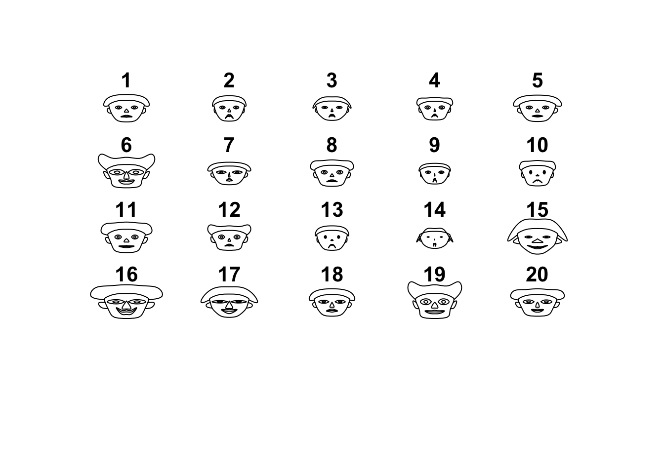
一般的Chernoff脸谱图是这样的,以R中自带的鸢尾花数据集(iris)为例:
library(aplpack)
faces(iris[1:20,1:4],face.type=0)
## effect of variables:
##  modified item       Var
##  "height of face   " "Sepal.Length"
##  "width of face    " "Sepal.Width"
##  "structure of face" "Petal.Length"
##  "height of mouth  " "Petal.Width"
##  "width of mouth   " "Sepal.Length"
##  "smiling          " "Sepal.Width"
##  "height of eyes   " "Petal.Length"
##  "width of eyes    " "Petal.Width"
##  "height of hair   " "Sepal.Length"
##  "width of hair   "  "Sepal.Width"
##  "style of hair   "  "Petal.Length"
##  "height of nose  "  "Petal.Width"
##  "width of nose   "  "Sepal.Length"
##  "width of ear    "  "Sepal.Width"
##  "height of ear   "  "Petal.Length"
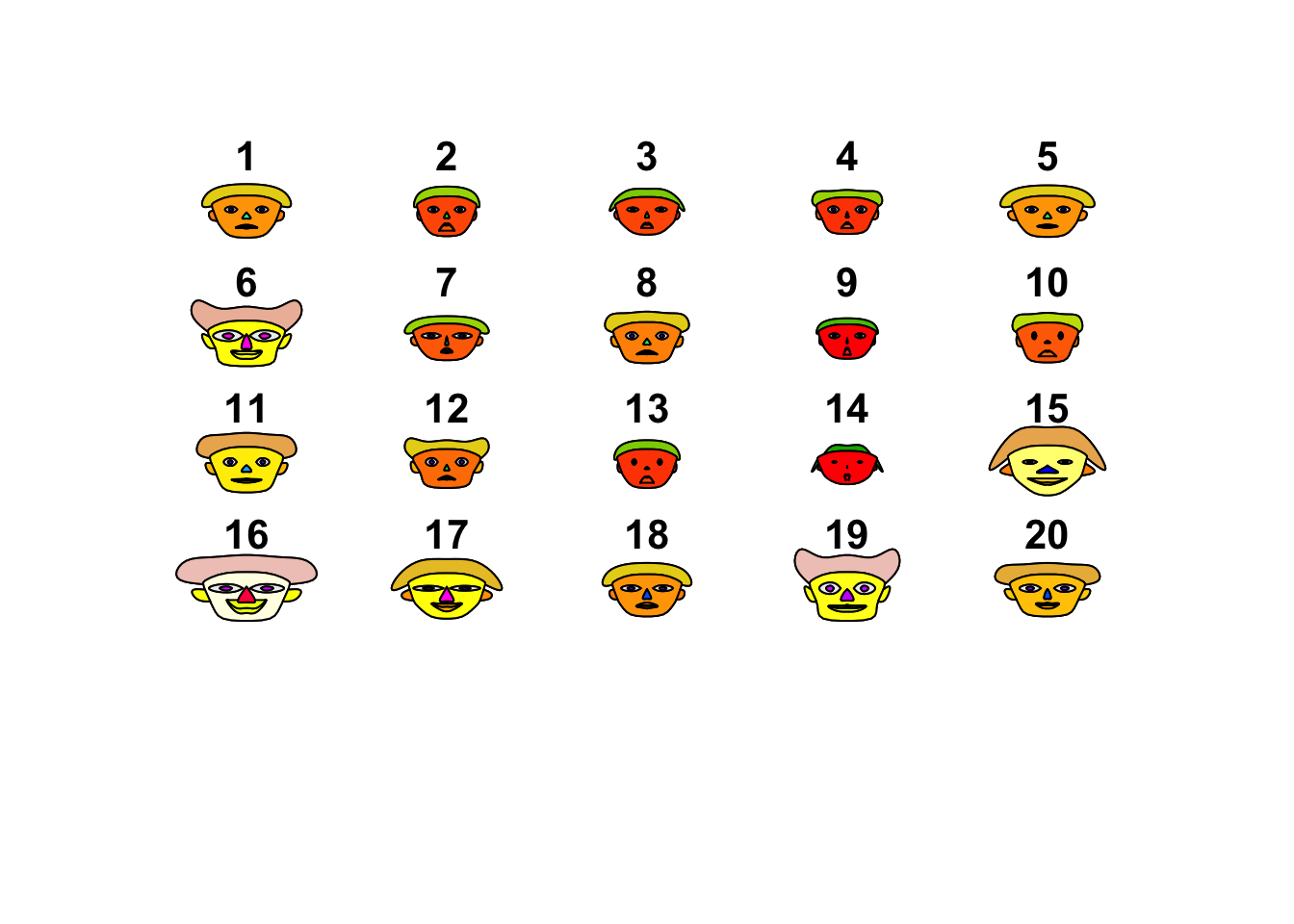
上图可能看起来比较呆板。我们当然可以画一个更好看的:
faces(iris[1:20,1:4],face.type=1)
## effect of variables:
##  modified item       Var
##  "height of face   " "Sepal.Length"
##  "width of face    " "Sepal.Width"
##  "structure of face" "Petal.Length"
##  "height of mouth  " "Petal.Width"
##  "width of mouth   " "Sepal.Length"
##  "smiling          " "Sepal.Width"
##  "height of eyes   " "Petal.Length"
##  "width of eyes    " "Petal.Width"
##  "height of hair   " "Sepal.Length"
##  "width of hair   "  "Sepal.Width"
##  "style of hair   "  "Petal.Length"
##  "height of nose  "  "Petal.Width"
##  "width of nose   "  "Sepal.Length"
##  "width of ear    "  "Sepal.Width"
##  "height of ear   "  "Petal.Length"
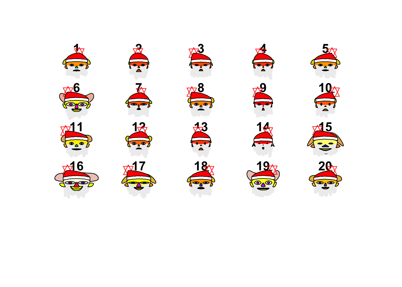
我比较喜欢圣诞老人这个版本:
faces(iris[1:20,1:4],face.type=2)
## effect of variables:
##  modified item       Var
##  "height of face   " "Sepal.Length"
##  "width of face    " "Sepal.Width"
##  "structure of face" "Petal.Length"
##  "height of mouth  " "Petal.Width"
##  "width of mouth   " "Sepal.Length"
##  "smiling          " "Sepal.Width"
##  "height of eyes   " "Petal.Length"
##  "width of eyes    " "Petal.Width"
##  "height of hair   " "Sepal.Length"
##  "width of hair   "  "Sepal.Width"
##  "style of hair   "  "Petal.Length"
##  "height of nose  "  "Petal.Width"
##  "width of nose   "  "Sepal.Length"
##  "width of ear    "  "Sepal.Width"
##  "height of ear   "  "Petal.Length"
主流多元数据可视化方法
虽然脸谱图看起来好玩儿有趣,但真正在业界落地数据可视化时,它并不太实用。业界有很多更加实用的多元数据可视化方法值得学习。这些方法大致可以分为以下几类:
基于几何的交互式方法
这类方法主要包括常用的散点图矩阵、平行坐标图和雷达图。
散点图矩阵
散点图以网格形式展示多个二维散点图,可以直观反映变量间的两两关系。适合探索变量之间的相关性,且可以通过颜色/符号增强信息表达的力度。
看一个例子:
# 加载包
library(GGally)
## 载入需要的程序包:ggplot2

## Registered S3 method overwritten by 'GGally':
##   method from
##   +.gg   ggplot2
# 绘制散点图矩阵(含密度图和相关系数)
ggpairs(iris, columns = 1:4,
        mapping = aes(color = Species),  # 按类别着色
        upper = list(continuous = "cor"),
        lower = list(continuous = "smooth"))
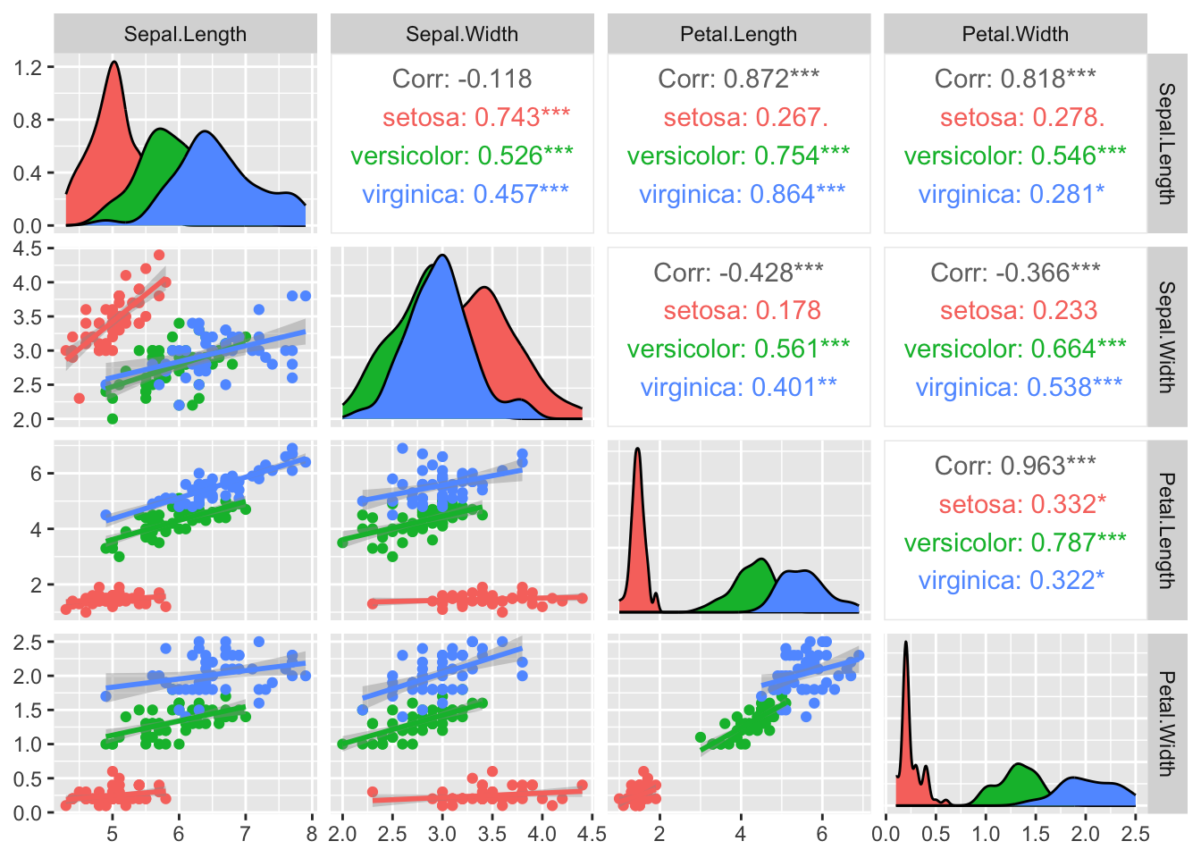
散点图矩阵的缺点也很突出,当变量很多时,图形阅读难度会大幅提升。
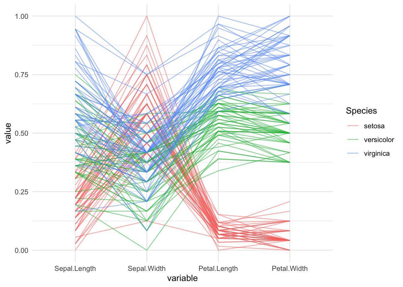
平行坐标图
通过平行排列的坐标轴进行多维数据可视化,图上以折线连接各变量值。它的优点是清晰呈现高维数据中的聚类、趋势和异常值。缺点是高维数据易导致线条重叠,需结合交互操作优。
上一个例子:
library(GGally)

# 绘制平行坐标图(标准化处理)
ggparcoord(iris, columns = 1:4, groupColumn = 5,
           scale = "uniminmax",  # 标准化到[0,1]
           alphaLines = 0.5) +
  theme_minimal()
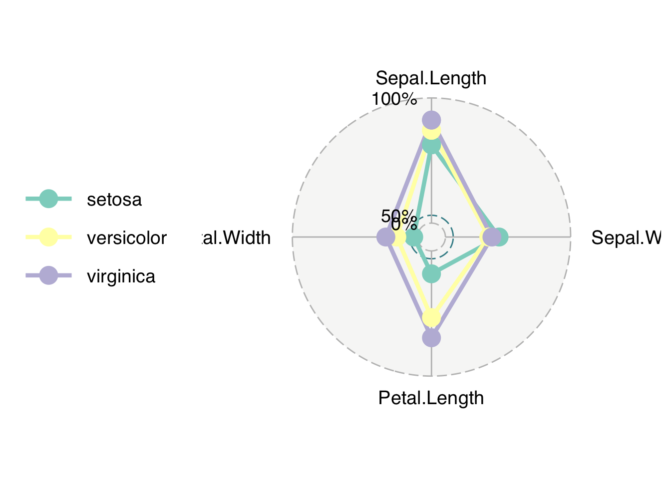
雷达图
雷达图在工业界和商业界应用广泛,它是以多边形闭合图形展示多维数据,用顶点代表变量值。雷达图适合多指标对比(如产品性能评估),缺点是数据差异较大时图形易失真。
# 安装包(如未安装)
# devtools::install_github("ricardo-bion/ggradar")

library(ggradar)
library(dplyr)
##
## 载入程序包:'dplyr'

## The following objects are masked from 'package:stats':
##
##     filter, lag

## The following objects are masked from 'package:base':
##
##     intersect, setdiff, setequal, union
# 数据预处理(计算各物种均值)
iris_radar <- iris %>%
  group_by(Species) %>%
  summarise(across(1:4, mean))

# 绘制雷达图
ggradar(iris_radar, grid.min = 0, grid.max = 8)
基于像素的密度表现方法
主要包括热力图和像素图。
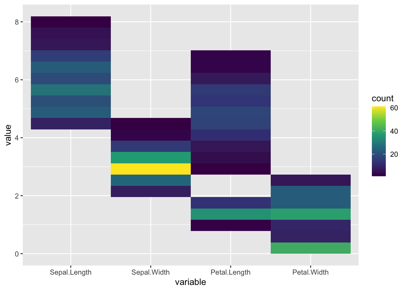
热力图
热力图以色块颜色深浅表示数值大小或分布密度。常用于展示数据矩阵的关联模式(如用户行为聚类)等。
library(ggplot2)
library(reshape2)

# 数据长格式转换
iris_melt <- melt(iris[,1:4])
## No id variables; using all as measure variables
# 绘制热力图(数值分布)
ggplot(iris_melt, aes(x = variable, y = value)) +
  geom_bin2d(bins = 20) +  # 二维密度统计
  scale_fill_viridis_c()    # 颜色渐变
像素图
像素图将数据映射为像素的颜色或亮度属性。适合大规模数据的高效呈现。
降维和空间映射方法
主要包括主成分分析方法、t-SNE与UMAP方法及气泡图。
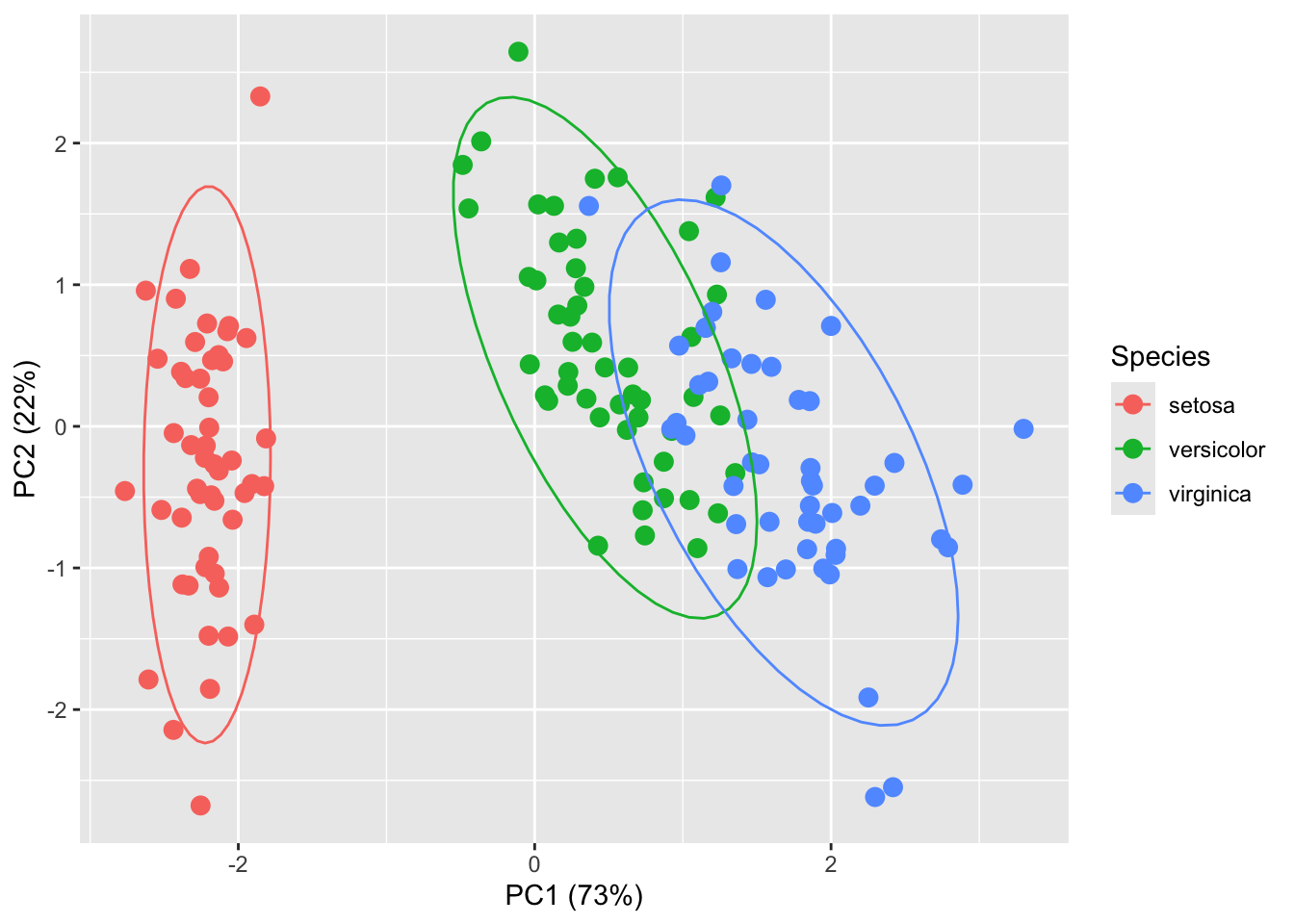
主成分分析(PCA)
PCA的思想是将高维数据投影到低维空间,保留主要方差信息,再在低维空间对数据进行可视化。
# PCA分析
pca <- prcomp(iris[,1:4], scale = TRUE)
pca_scores <- data.frame(pca$x, Species = iris$Species)

# 绘制PCA二维投影
ggplot(pca_scores, aes(x = PC1, y = PC2, color = Species)) +
  geom_point(size = 3) +
  stat_ellipse(level = 0.95) +  # 添加置信椭圆
  labs(x = "PC1 (73%)", y = "PC2 (22%)")  # 方差解释率
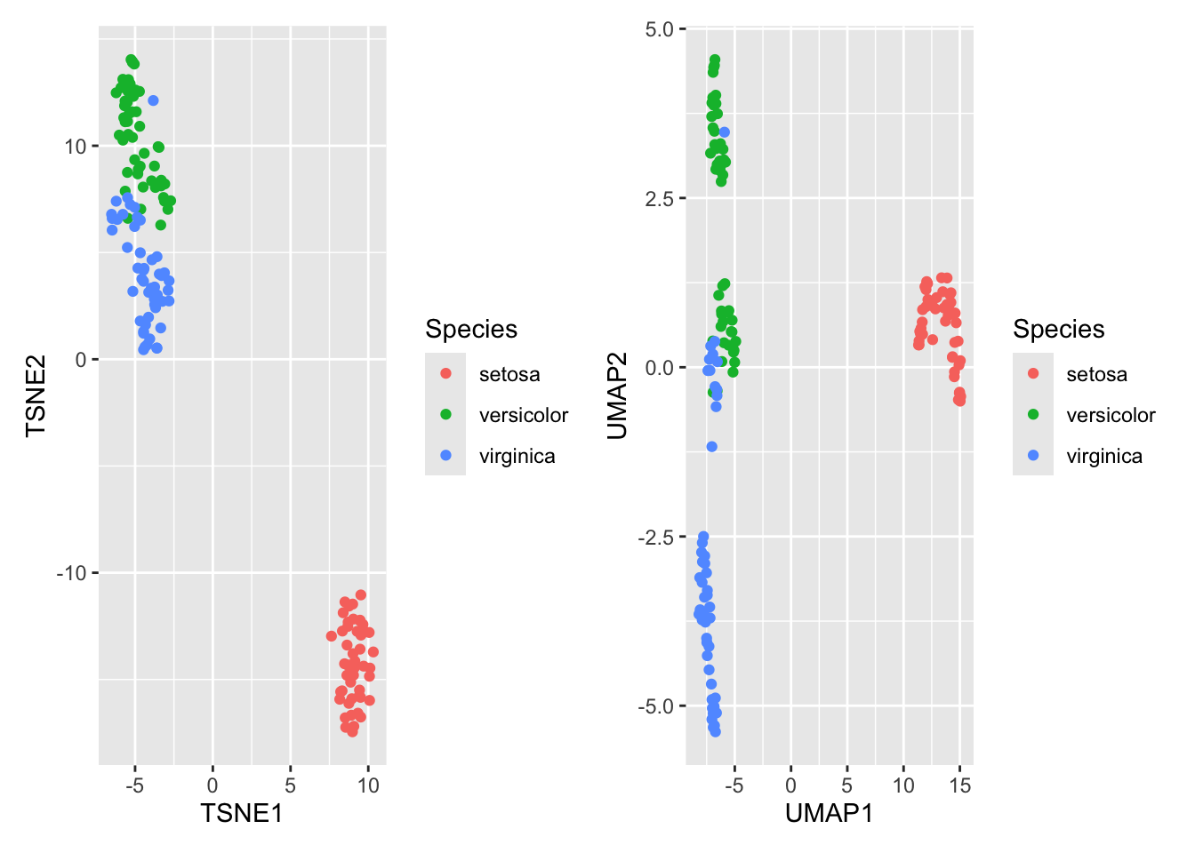
t-SNE与UMAP方法
这两种方法都是非线性降维方法,更擅长保留局部结构和聚类特征。
# t-SNE
library(Rtsne)
set.seed(123)
iris <- unique(iris)
tsne <- Rtsne(unique(iris[,1:4]), perplexity = 30)
tsne_df <- data.frame(TSNE1 = tsne$Y[,1], TSNE2 = tsne$Y[,2], Species = iris$Species)

# UMAP
library(umap)
umap_res <- umap(iris[,1:4])
umap_df <- data.frame(UMAP1 = umap_res$layout[,1], UMAP2 = umap_res$layout[,2], Species = iris$Species)

# 可视化对比
library(patchwork)
p1 <- ggplot(tsne_df, aes(TSNE1, TSNE2, color = Species)) + geom_point()
p2 <- ggplot(umap_df, aes(UMAP1, UMAP2, color = Species)) + geom_point()
p1 + p2  # 并排显示
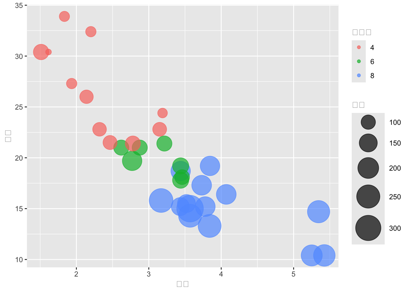
气泡图
library(ggplot2)
ggplot(mtcars, aes(x = wt, y = mpg, size = hp, color = factor(cyl))) +
  geom_point(alpha = 0.7) +
  scale_size(range = c(3, 15)) +  # 调整气泡尺寸范围
  labs(x = "车重", y = "油耗", color = "气缸数", size = "马力")
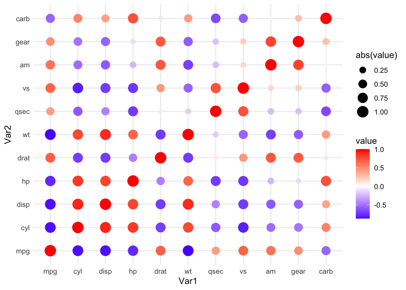
气泡图可以和热图相结合。
library(reshape2)
data_melt <- melt(cor(mtcars))  # 数据长格式转换

p <- ggplot(data_melt, aes(Var1, Var2, size = abs(value), color = value)) +
  geom_point() +
  scale_color_gradient2(low = "blue", mid = "white", high = "red") +  # 渐变色
  theme_minimal()
p
气泡图还可以变成交互式的。
library(plotly)
##
## 载入程序包:'plotly'

## The following object is masked from 'package:ggplot2':
##
##     last_plot

## The following object is masked from 'package:stats':
##
##     filter

## The following object is masked from 'package:graphics':
##
##     layout
ggplotly(p) # 将静态ggplot转换为交互式图表
其他方法
主要包括桑基图、三维散点图和表格透镜。
桑基图
这是一个垂直领域的多元数据可视化的方法,它可以展示流量或资源在多节点间的流转路径(如用户转化漏斗)。
# 安装包(如未安装)
# devtools::install_github("https://github.com/christophergandrud/networkD3")
library(networkD3)

# 构造示例数据(模拟物种间转化)
nodes <- data.frame(name = c("Setosa", "Versicolor", "Virginica"))
links <- data.frame(source = c(0,1,2), target = c(1,2,0), value = c(10,20,15))

# 绘制桑基图
sankeyNetwork(Links = links, Nodes = nodes,
              Source = "source", Target = "target",
              Value = "value", NodeID = "name")
三维散点图
通过三维空间扩展,直观呈现三个变量间的关系。
library(plotly)

# 交互式三维散点图
plot_ly(iris, x = ~Sepal.Length, y = ~Sepal.Width, z = ~Petal.Length,
        color = ~Species, type = "scatter3d", mode = "markers")
表格透镜
以交互式表格结合横条/点状图,快速比较大量数据与属性。
library(gt)
library(gtExtras)
# 创建交互式表格(含条形图)
iris %>%
  gt() %>%
  gt_plt_bar(column = Sepal.Length, width = 50) %>%  # 添加条形图
  gt_theme_nytimes()  # 主题风格
| Sepal.Length | Sepal.Width | Petal.Length | Petal.Width | Species |
|---|---|---|---|---|
| 3.5 | 1.4 | 0.2 | setosa | |
| 3.0 | 1.4 | 0.2 | setosa | |
| 3.2 | 1.3 | 0.2 | setosa | |
| 3.1 | 1.5 | 0.2 | setosa | |
| 3.6 | 1.4 | 0.2 | setosa | |
| 3.9 | 1.7 | 0.4 | setosa | |
| 3.4 | 1.4 | 0.3 | setosa | |
| 3.4 | 1.5 | 0.2 | setosa | |
| 2.9 | 1.4 | 0.2 | setosa | |
| 3.1 | 1.5 | 0.1 | setosa | |
| 3.7 | 1.5 | 0.2 | setosa | |
| 3.4 | 1.6 | 0.2 | setosa | |
| 3.0 | 1.4 | 0.1 | setosa | |
| 3.0 | 1.1 | 0.1 | setosa | |
| 4.0 | 1.2 | 0.2 | setosa | |
| 4.4 | 1.5 | 0.4 | setosa | |
| 3.9 | 1.3 | 0.4 | setosa | |
| 3.5 | 1.4 | 0.3 | setosa | |
| 3.8 | 1.7 | 0.3 | setosa | |
| 3.8 | 1.5 | 0.3 | setosa | |
| 3.4 | 1.7 | 0.2 | setosa | |
| 3.7 | 1.5 | 0.4 | setosa | |
| 3.6 | 1.0 | 0.2 | setosa | |
| 3.3 | 1.7 | 0.5 | setosa | |
| 3.4 | 1.9 | 0.2 | setosa | |
| 3.0 | 1.6 | 0.2 | setosa | |
| 3.4 | 1.6 | 0.4 | setosa | |
| 3.5 | 1.5 | 0.2 | setosa | |
| 3.4 | 1.4 | 0.2 | setosa | |
| 3.2 | 1.6 | 0.2 | setosa | |
| 3.1 | 1.6 | 0.2 | setosa | |
| 3.4 | 1.5 | 0.4 | setosa | |
| 4.1 | 1.5 | 0.1 | setosa | |
| 4.2 | 1.4 | 0.2 | setosa | |
| 3.1 | 1.5 | 0.2 | setosa | |
| 3.2 | 1.2 | 0.2 | setosa | |
| 3.5 | 1.3 | 0.2 | setosa | |
| 3.6 | 1.4 | 0.1 | setosa | |
| 3.0 | 1.3 | 0.2 | setosa | |
| 3.4 | 1.5 | 0.2 | setosa | |
| 3.5 | 1.3 | 0.3 | setosa | |
| 2.3 | 1.3 | 0.3 | setosa | |
| 3.2 | 1.3 | 0.2 | setosa | |
| 3.5 | 1.6 | 0.6 | setosa | |
| 3.8 | 1.9 | 0.4 | setosa | |
| 3.0 | 1.4 | 0.3 | setosa | |
| 3.8 | 1.6 | 0.2 | setosa | |
| 3.2 | 1.4 | 0.2 | setosa | |
| 3.7 | 1.5 | 0.2 | setosa | |
| 3.3 | 1.4 | 0.2 | setosa | |
| 3.2 | 4.7 | 1.4 | versicolor | |
| 3.2 | 4.5 | 1.5 | versicolor | |
| 3.1 | 4.9 | 1.5 | versicolor | |
| 2.3 | 4.0 | 1.3 | versicolor | |
| 2.8 | 4.6 | 1.5 | versicolor | |
| 2.8 | 4.5 | 1.3 | versicolor | |
| 3.3 | 4.7 | 1.6 | versicolor | |
| 2.4 | 3.3 | 1.0 | versicolor | |
| 2.9 | 4.6 | 1.3 | versicolor | |
| 2.7 | 3.9 | 1.4 | versicolor | |
| 2.0 | 3.5 | 1.0 | versicolor | |
| 3.0 | 4.2 | 1.5 | versicolor | |
| 2.2 | 4.0 | 1.0 | versicolor | |
| 2.9 | 4.7 | 1.4 | versicolor | |
| 2.9 | 3.6 | 1.3 | versicolor | |
| 3.1 | 4.4 | 1.4 | versicolor | |
| 3.0 | 4.5 | 1.5 | versicolor | |
| 2.7 | 4.1 | 1.0 | versicolor | |
| 2.2 | 4.5 | 1.5 | versicolor | |
| 2.5 | 3.9 | 1.1 | versicolor | |
| 3.2 | 4.8 | 1.8 | versicolor | |
| 2.8 | 4.0 | 1.3 | versicolor | |
| 2.5 | 4.9 | 1.5 | versicolor | |
| 2.8 | 4.7 | 1.2 | versicolor | |
| 2.9 | 4.3 | 1.3 | versicolor | |
| 3.0 | 4.4 | 1.4 | versicolor | |
| 2.8 | 4.8 | 1.4 | versicolor | |
| 3.0 | 5.0 | 1.7 | versicolor | |
| 2.9 | 4.5 | 1.5 | versicolor | |
| 2.6 | 3.5 | 1.0 | versicolor | |
| 2.4 | 3.8 | 1.1 | versicolor | |
| 2.4 | 3.7 | 1.0 | versicolor | |
| 2.7 | 3.9 | 1.2 | versicolor | |
| 2.7 | 5.1 | 1.6 | versicolor | |
| 3.0 | 4.5 | 1.5 | versicolor | |
| 3.4 | 4.5 | 1.6 | versicolor | |
| 3.1 | 4.7 | 1.5 | versicolor | |
| 2.3 | 4.4 | 1.3 | versicolor | |
| 3.0 | 4.1 | 1.3 | versicolor | |
| 2.5 | 4.0 | 1.3 | versicolor | |
| 2.6 | 4.4 | 1.2 | versicolor | |
| 3.0 | 4.6 | 1.4 | versicolor | |
| 2.6 | 4.0 | 1.2 | versicolor | |
| 2.3 | 3.3 | 1.0 | versicolor | |
| 2.7 | 4.2 | 1.3 | versicolor | |
| 3.0 | 4.2 | 1.2 | versicolor | |
| 2.9 | 4.2 | 1.3 | versicolor | |
| 2.9 | 4.3 | 1.3 | versicolor | |
| 2.5 | 3.0 | 1.1 | versicolor | |
| 2.8 | 4.1 | 1.3 | versicolor | |
| 3.3 | 6.0 | 2.5 | virginica | |
| 2.7 | 5.1 | 1.9 | virginica | |
| 3.0 | 5.9 | 2.1 | virginica | |
| 2.9 | 5.6 | 1.8 | virginica | |
| 3.0 | 5.8 | 2.2 | virginica | |
| 3.0 | 6.6 | 2.1 | virginica | |
| 2.5 | 4.5 | 1.7 | virginica | |
| 2.9 | 6.3 | 1.8 | virginica | |
| 2.5 | 5.8 | 1.8 | virginica | |
| 3.6 | 6.1 | 2.5 | virginica | |
| 3.2 | 5.1 | 2.0 | virginica | |
| 2.7 | 5.3 | 1.9 | virginica | |
| 3.0 | 5.5 | 2.1 | virginica | |
| 2.5 | 5.0 | 2.0 | virginica | |
| 2.8 | 5.1 | 2.4 | virginica | |
| 3.2 | 5.3 | 2.3 | virginica | |
| 3.0 | 5.5 | 1.8 | virginica | |
| 3.8 | 6.7 | 2.2 | virginica | |
| 2.6 | 6.9 | 2.3 | virginica | |
| 2.2 | 5.0 | 1.5 | virginica | |
| 3.2 | 5.7 | 2.3 | virginica | |
| 2.8 | 4.9 | 2.0 | virginica | |
| 2.8 | 6.7 | 2.0 | virginica | |
| 2.7 | 4.9 | 1.8 | virginica | |
| 3.3 | 5.7 | 2.1 | virginica | |
| 3.2 | 6.0 | 1.8 | virginica | |
| 2.8 | 4.8 | 1.8 | virginica | |
| 3.0 | 4.9 | 1.8 | virginica | |
| 2.8 | 5.6 | 2.1 | virginica | |
| 3.0 | 5.8 | 1.6 | virginica | |
| 2.8 | 6.1 | 1.9 | virginica | |
| 3.8 | 6.4 | 2.0 | virginica | |
| 2.8 | 5.6 | 2.2 | virginica | |
| 2.8 | 5.1 | 1.5 | virginica | |
| 2.6 | 5.6 | 1.4 | virginica | |
| 3.0 | 6.1 | 2.3 | virginica | |
| 3.4 | 5.6 | 2.4 | virginica | |
| 3.1 | 5.5 | 1.8 | virginica | |
| 3.0 | 4.8 | 1.8 | virginica | |
| 3.1 | 5.4 | 2.1 | virginica | |
| 3.1 | 5.6 | 2.4 | virginica | |
| 3.1 | 5.1 | 2.3 | virginica | |
| 3.2 | 5.9 | 2.3 | virginica | |
| 3.3 | 5.7 | 2.5 | virginica | |
| 3.0 | 5.2 | 2.3 | virginica | |
| 2.5 | 5.0 | 1.9 | virginica | |
| 3.0 | 5.2 | 2.0 | virginica | |
| 3.4 | 5.4 | 2.3 | virginica | |
| 3.0 | 5.1 | 1.8 | virginica |
以上所有这些方法也同样可以用于经济数据、财务数据和股票数据的可视化。