scatterplot3d是一个力图在3D空间展示多维数据的R包,在这个包里只含有一个函数scatterplot3d(),这一点上可谓是特立独行。scatterplot3d()的用法如下:
    scatterplot3d(x, y=NULL, z=NULL, color=par("col"), pch=NULL,
        main=NULL, sub=NULL, xlim=NULL, ylim=NULL, zlim=NULL,
        xlab=NULL, ylab=NULL, zlab=NULL, scale.y=1, angle=40,
        axis=TRUE, tick.marks=TRUE, label.tick.marks=TRUE,
        x.ticklabs=NULL, y.ticklabs=NULL, z.ticklabs=NULL,
        y.margin.add=0, grid=TRUE, box=TRUE, lab=par("lab"),
        lab.z=mean(lab[1:2]), type="p", highlight.3d=FALSE,
        mar=c(5,3,4,3)+0.1, col.axis=par("col.axis"),
        col.grid="grey", col.lab=par("col.lab"),
        cex.symbols=par("cex"), cex.axis=0.8 * par("cex.axis"),
        cex.lab=par("cex.lab"), font.axis=par("font.axis"),
        font.lab=par("font.lab"), lty.axis=par("lty"),
        lty.grid=par("lty"), lty.hide=NULL, lty.hplot=par("lty"),
        log="", ...)
这个函数的参数多到让人眼花缭乱。下面是几个例子:
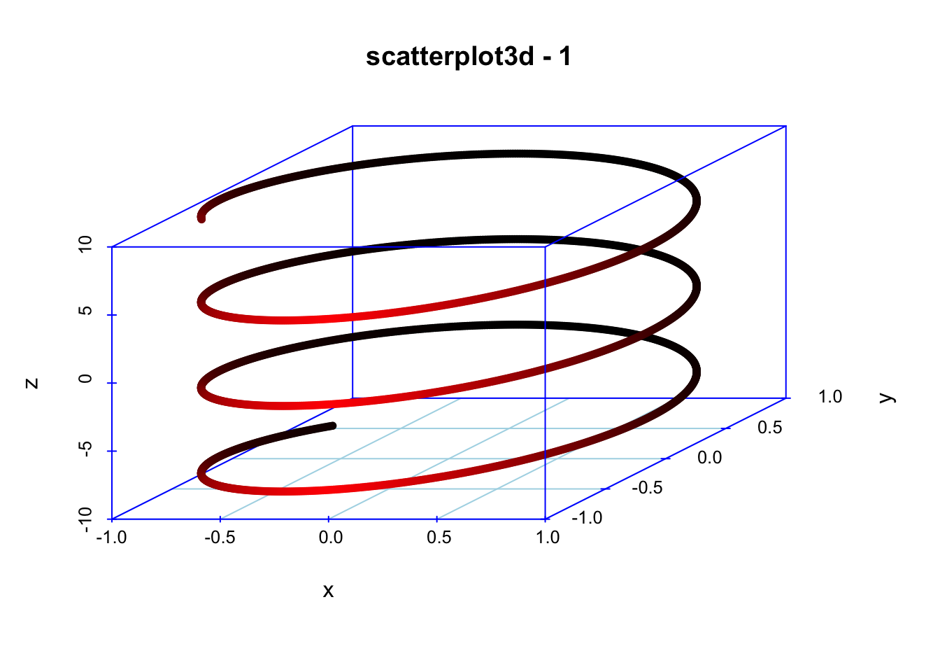
先用scatterplot3d()画一个螺旋线:
library(scatterplot3d)
z <- seq(-10, 10, 0.01)
x <- cos(z)
y <- sin(z)
scatterplot3d(x, y, z, highlight.3d=TRUE, col.axis="blue",col.grid="lightblue",main="scatterplot3d - 1", pch=20)
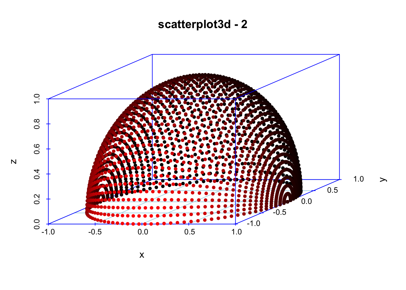
再画半椭圆:
temp<- seq(-pi, 0, length = 50)
x <- c(rep(1, 50) %*% t(cos(temp)))
y <- c(cos(temp) %*% t(sin(temp)))
z <- c(sin(temp) %*% t(sin(temp)))
scatterplot3d(x, y, z, highlight.3d=TRUE,col.axis="blue", col.grid="lightblue",main="scatterplot3d - 2", pch=20)
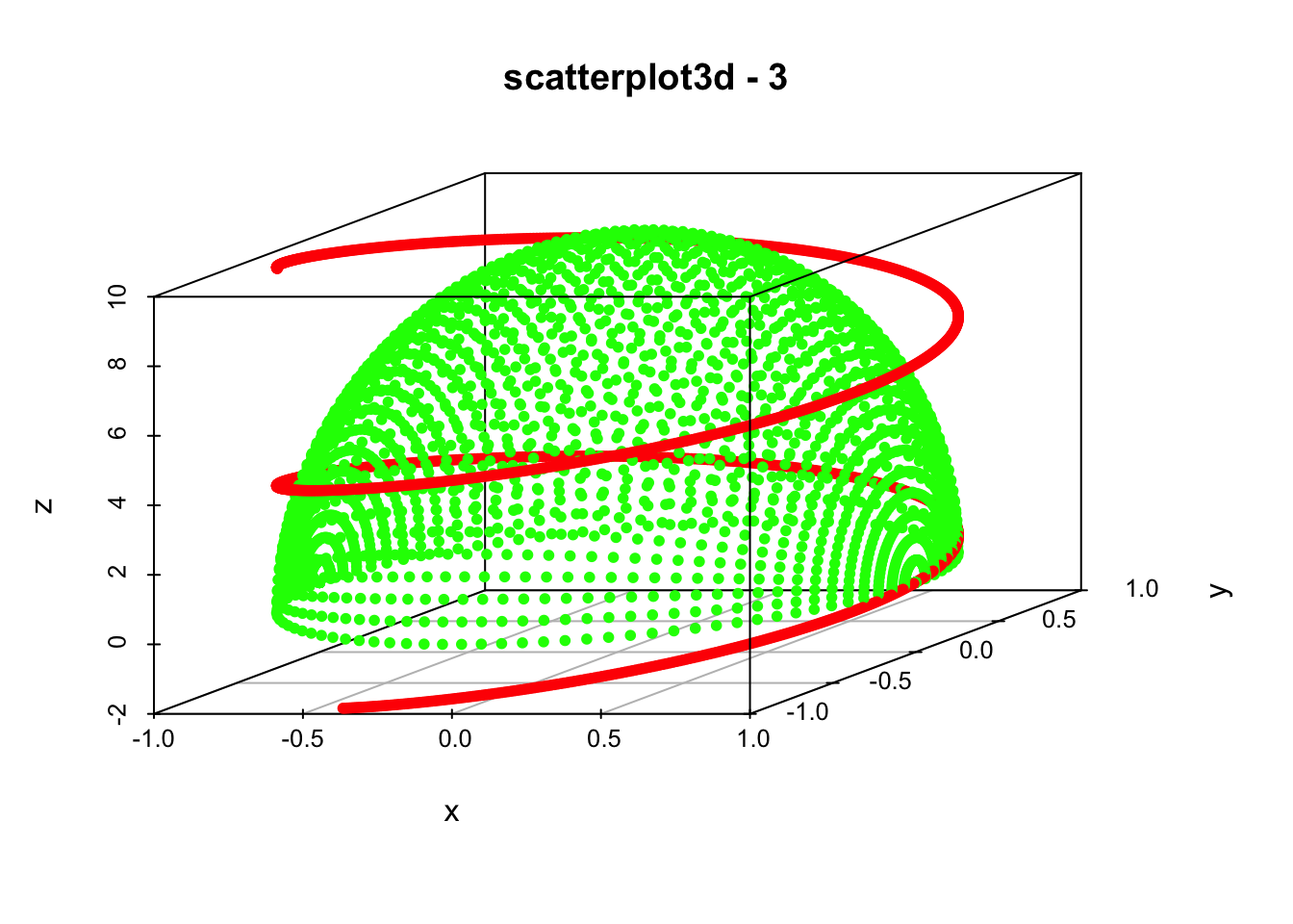
将两者结合,输出结果很像龙盘柱。有点酷!
    x <- c(rep(1, 50) %*% t(cos(temp)))
    y <- c(cos(temp) %*% t(sin(temp)))
    z <- 10 * c(sin(temp) %*% t(sin(temp)))
    color <- rep("green", length(x))
    temp <- seq(-10, 10, 0.01)
    x <- c(x, cos(temp))
    y <- c(y, sin(temp))
    z <- c(z, temp)
    color <- c(color, rep("red", length(temp)))
    scatterplot3d(x, y, z, color, pch=20, zlim=c(-2, 10),main="scatterplot3d - 3")
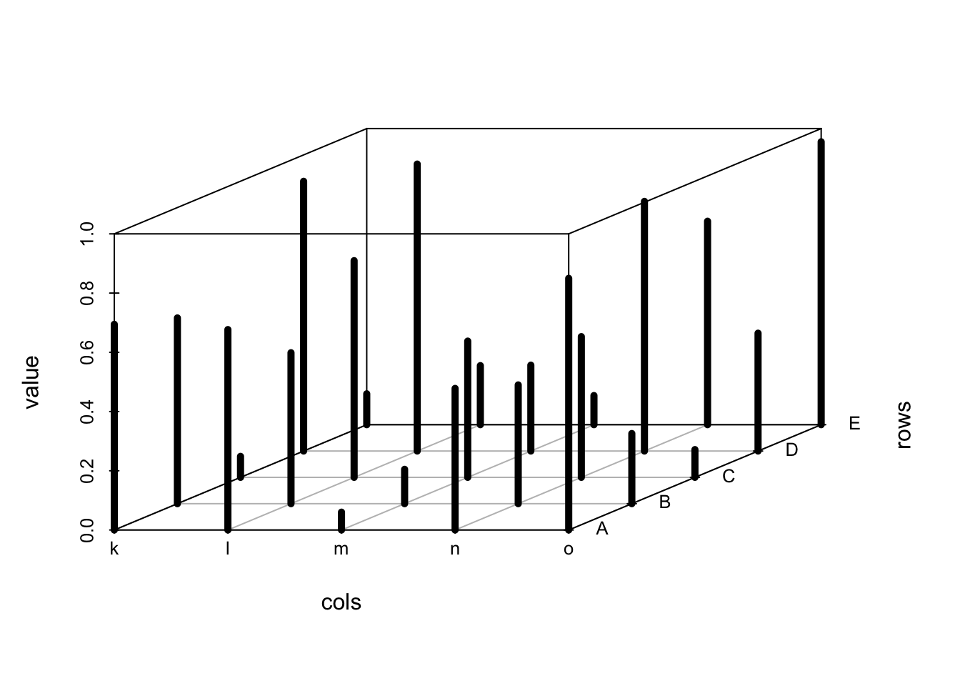
来一个比较庸俗的,三维bar图:
my.mat <- matrix(runif(25), nrow=5)
dimnames(my.mat) <- list(LETTERS[1:5], letters[11:15])
s3d.dat <- data.frame(cols=as.vector(col(my.mat)),rows=as.vector(row(my.mat)),value=as.vector(my.mat))
scatterplot3d(s3d.dat, type="h", lwd=5, pch=" ",x.ticklabs=colnames(my.mat),y.ticklabs=rownames(my.mat))
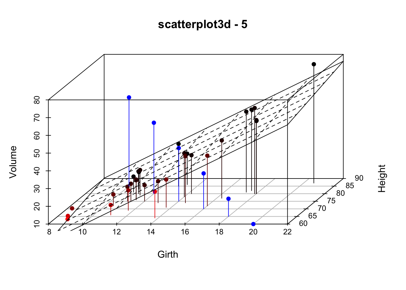
上面的可以说都不是很实用,下面看一下二维回归平面图:
data(trees)
s3d <- scatterplot3d(trees, type="h", highlight.3d=TRUE,angle=55, scale.y=0.7, pch=16, main="scatterplot3d - 5")
s3d$points3d(seq(10,20,2), seq(85,60,-5), seq(60,10,-10),col="blue", type="h", pch=16)
     # 画回归平面
attach(trees)
my.lm <- lm(Volume ~ Girth + Height)
s3d$plane3d(my.lm, lty.box = "solid")
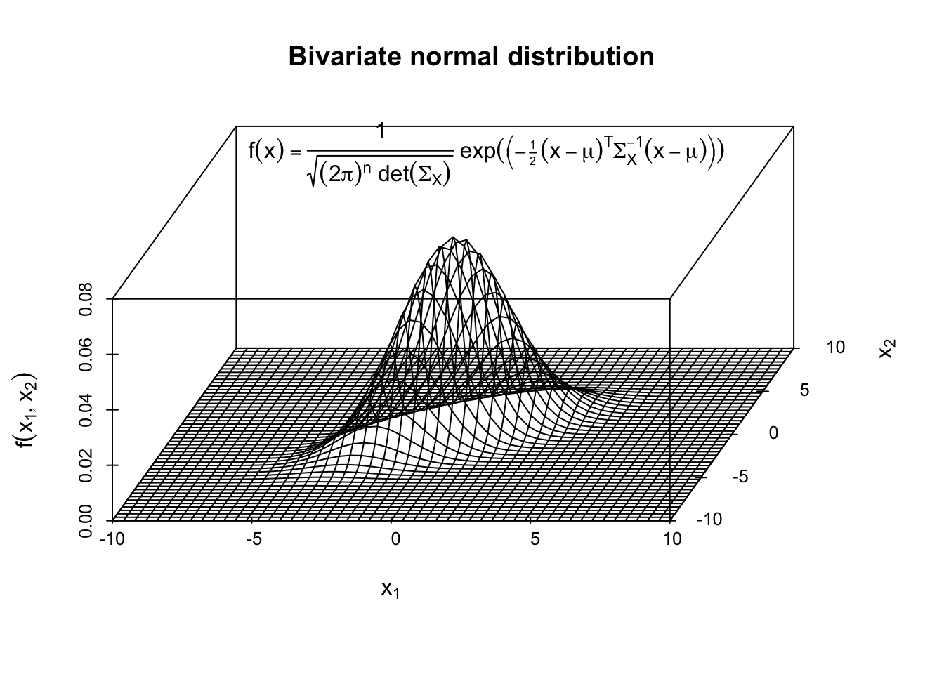
我看见有很多帖子索要二维正态分布的示意图,这里画一个,
     library(mvtnorm)
     x1 <- seq(-10, 10, length = 51)
     x2 <- seq(-10, 10, length = 51)
     dens <- matrix(dmvnorm(expand.grid(x1,x2),sigma=rbind(c(3,2),c(2,3))),ncol=length(x1))
     s3d<-scatterplot3d(x1,x2,seq(min(dens),max(dens),length=length(x1)),
     type="n",grid=FALSE,angle = 70,
     zlab=expression(f(x[1],x[2])),
     xlab=expression(x[1]),ylab=expression(x[2]),
     main="Bivariate normal distribution")
     text(s3d$xyz.convert(-1,10,0.07),
    labels=expression(f(x)==frac(1,sqrt((2*pi)^n*phantom(".")*det(Sigma[X])))*phantom(".")*exp(bgroup("(",-scriptstyle(frac(1,2)*phantom("."))*(x-mu)^T*Sigma[X]^-1*(x-mu),")"))))
     for(i in length(x1):1)
     s3d$points3d(rep(x1[i], length(x2)), x2, dens[i,], type = "l")
     for(i in length(x2):1)
     s3d$points3d(x1, rep(x2[i], length(x1)), dens[,i], type = "l")
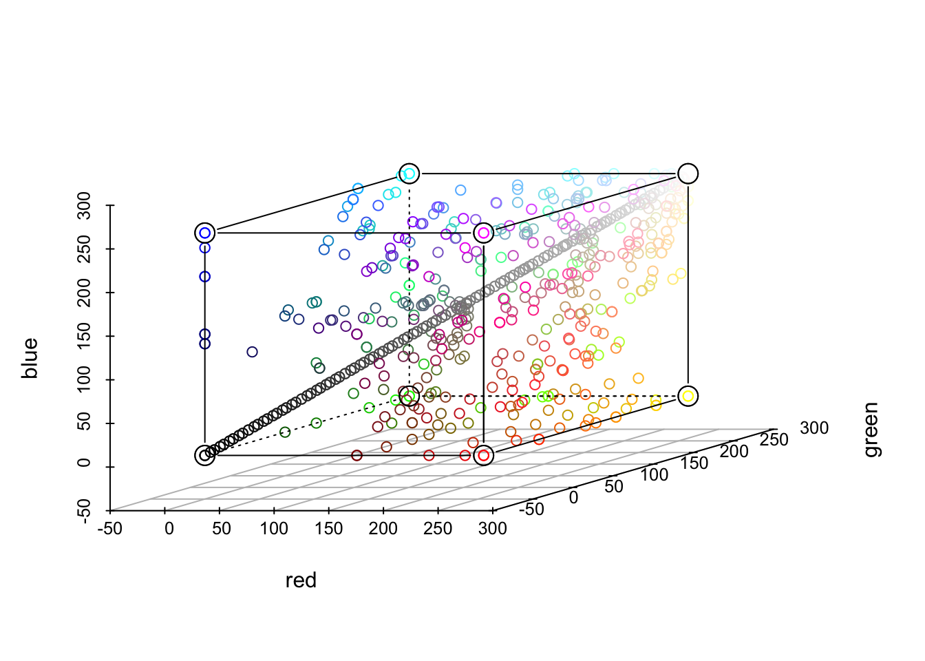
之所以画下面这个,完全是因为我贪图色彩:
     cubedraw <- function(res3d, min = 0, max = 255, cex = 2, text. = FALSE)
       {
         cube01 <- rbind(c(0,0,1), 0, c(1,0,0), c(1,1,0), 1, c(0,1,1), # < 6 outer
                         c(1,0,1), c(0,1,0))
         cub <- min + (max-min)* cube01
         res3d$points3d(cub[c(1:6,1,7,3,7,5) ,], cex = cex, type = 'b', lty = 1)
         res3d$points3d(cub[c(2,8,4,8,6),     ], cex = cex, type = 'b', lty = 3)
         if(text.)
             text(res3d$xyz.convert(cub), labels=1:nrow(cub), col='tomato', cex=2)
       }
       cc <- colors()
       crgb <- t(col2rgb(cc))
       par(xpd = TRUE)
       rr <- scatterplot3d(crgb, color = cc, box = FALSE, angle = 24,
           xlim = c(-50, 300), ylim = c(-50, 300), zlim = c(-50, 300))
       cubedraw(rr)
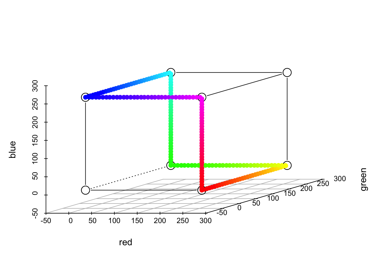
       rbc <- rainbow(201)
       Rrb <- t(col2rgb(rbc))
       rR <- scatterplot3d(Rrb, color = rbc, box = FALSE, angle = 24,
           xlim = c(-50, 300), ylim = c(-50, 300), zlim = c(-50, 300))
       cubedraw(rR)
       rR$points3d(Rrb, col = rbc, pch = 16)