蒙特卡洛模拟法
蒙特卡洛模拟法是一种基于随机抽样和统计模拟的数值计算方法,其通过生成大量随机样本,利用概率统计理论估计复杂问题的近似解。该方法由数学家冯·诺伊曼和乌拉姆于20世纪40年代在核武器研制项目中首次提出。蒙特卡洛模拟法也可以用来计算投资组合的VaR。
在应用蒙特卡洛模拟法计算VaR时,首先根据投资组合的历史特征,总结投资组合收益率对应的可能分布并提取该分布对应的核心参数;再以这些核心参数为基础,结合特定分布模拟出一系列符合要求的伪随机数作为假想的未来数据;最后,以这些“假想的未来数据”作为研究对象计算出VaR值。
蒙特卡洛模拟法计算单资产VaR
基于R语言应用蒙特卡洛模拟法计算VaR的代码如下:
# 加载必要包
if (!require("quantmod")) install.packages("quantmod")
## 载入需要的程序包:quantmod
## 载入需要的程序包:xts
## 载入需要的程序包:zoo
##
## 载入程序包:'zoo'
## The following objects are masked from 'package:base':
##
##     as.Date, as.Date.numeric
## 载入需要的程序包:TTR
## Registered S3 method overwritten by 'quantmod':
##   method            from
##   as.zoo.data.frame zoo
if (!require("MASS")) install.packages("MASS")
## 载入需要的程序包:MASS
library(quantmod)
library(MASS)
library(dplyr)
##
## ######################### Warning from 'xts' package ##########################
## #                                                                             #
## # The dplyr lag() function breaks how base R's lag() function is supposed to  #
## # work, which breaks lag(my_xts). Calls to lag(my_xts) that you type or       #
## # source() into this session won't work correctly.                            #
## #                                                                             #
## # Use stats::lag() to make sure you're not using dplyr::lag(), or you can add #
## # conflictRules('dplyr', exclude = 'lag') to your .Rprofile to stop           #
## # dplyr from breaking base R's lag() function.                                #
## #                                                                             #
## # Code in packages is not affected. It's protected by R's namespace mechanism #
## # Set `options(xts.warn_dplyr_breaks_lag = FALSE)` to suppress this warning.  #
## #                                                                             #
## ###############################################################################
##
## 载入程序包:'dplyr'
## The following object is masked from 'package:MASS':
##
##     select
## The following objects are masked from 'package:xts':
##
##     first, last
## The following objects are masked from 'package:stats':
##
##     filter, lag
## The following objects are masked from 'package:base':
##
##     intersect, setdiff, setequal, union
# 获取苹果公司股票数据(过去2年)
getSymbols("AAPL", src = "yahoo", from = as.Date("2023-05-01"), to = as.Date(Sys.Date()))
## [1] "AAPL"
# 计算对数收益率
returns <- na.omit(ROC(Cl(AAPL)))
colnames(returns) <- "AAPL_Return"
# 参数设置
set.seed(123)
n_sim <- 10000 # 模拟次数
confidence_level <- 0.95
portfolio_value <- 1e6 # 组合价值100万美元
# 估计收益率参数
mu <- mean(returns)
sigma <- sd(returns)
# 蒙特卡洛模拟(正态分布)
sim_normal <- rnorm(n_sim, mean = mu, sd = sigma)
portfolio_loss_normal <- portfolio_value * (1 - exp(sim_normal)) # 对数收益转换为价格变动
# 蒙特卡洛模拟(t分布)
# 计算VaR
var_normal <- quantile(portfolio_loss_normal, probs = confidence_level)
# 格式化输出
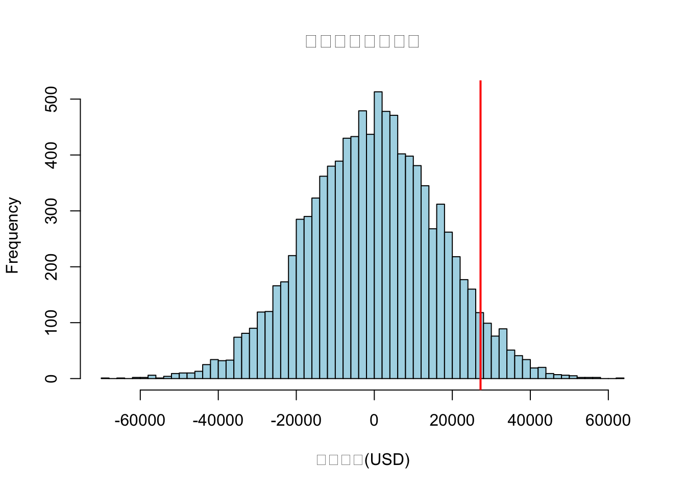
cat("蒙特卡洛模拟VaR(正态分布假设):", round(var_normal, 2), "USD\n")
## 蒙特卡洛模拟VaR(正态分布假设): 27011.97 USD
# 可视化比较
hist(portfolio_loss_normal, breaks = 50, main = "正态分布模拟损失",
     xlab = "损失金额(USD)", col = "lightblue")
abline(v = var_normal, col = "red", lwd = 2)
也可以将模拟的分布确定为以下分布:
- 偏正态分布
- 偏t分布
- 广义误差分布
- 偏广义误差分布
- 混合正态分布
蒙特卡洛模拟计算多资产投资组合VaR
蒙特卡洛模拟通过以下步骤实现多资产VaR计算:
- 历史数据获取:通过quantmod获取真实资产价格数据
- 参数估计:计算资产收益率的均值向量和协方差矩阵
- 路径生成:生成服从多元正态分布的模拟收益率路径
- 组合估值:根据权重计算组合价值变化
- 损失分布:统计模拟损失的分位数得到VaR
## 环境配置与数据获取
# ----------------------
# 加载必要包
# ----------------------
library(ggplot2)
# library(foreach)
# library(doParallel)
library(Matrix)
library(matrixcalc)

# ----------------------
# 参数设置
# ----------------------
symbols <- c("AAPL", "GOOG", "MSFT", "AMZN")  # 资产列表
weights <- c(0.3, 0.3, 0.2, 0.2)              # 投资权重
V0 <- 1000000                                 # 初始组合价值(美元)
n_sim <- 100000                               # 模拟次数
alpha <- 0.99                                 # 置信水平
T_days <- 10                                  # 持有期(天)
start_date <- "2020-01-01"
end_date <- format(Sys.Date(), "%Y-%m-%d")    # 动态获取最新数据

# ----------------------
# 获取真实历史数据
# ----------------------
getSymbols(symbols, src = "yahoo", from = start_date, to = end_date)
## [1] "AAPL" "GOOG" "MSFT" "AMZN"
# 提取调整后收盘价并计算日收益率
prices <- do.call(merge, lapply(symbols, function(x) Ad(get(x))))
# 替换原returns计算代码
returns <- ROC(prices, type = "discrete")
# 添加数据清洗
returns<- apply(returns, 2, function(x) {
x[is.infinite(x)] <- NA
na.omit(x)
})
# 验证数据完整性
if (any(is.na(returns)) || any(is.infinite(returns))) {
stop("数据清洗失败,仍存在缺失值或无穷值")
}
## 参数估计与路径生成(增强)
# ----------------------
# 计算统计参数(带时间调整)
# ----------------------
mu <- colMeans(returns) * T_days # 持有期收益率均值
sigma <- cov(returns) * T_days
robust_sigma <- function(sigma, eps=1e-8) {
eig <- eigen(sigma)
ev <- pmax(eig$values, eps) # 特征值下限保护
sigma_robust <- eig$vectors %*% diag(ev) %*% t(eig$vectors)
return(as.matrix(nearPD(sigma_robust, keepDiag=TRUE)$mat))
}
sigma <- robust_sigma(sigma)
# 协方差矩阵正定性修正
# 矩阵条件数校验
if (kappa(sigma) > 1e6) warning("协方差矩阵条件数过高,建议降维处理")
# 特征值范围验证
eigen_values <- eigen(sigma)$values
if (min(eigen_values) < 1e-6) stop("矩阵修正失败")
# ----------------------
# 蒙特卡洛模拟
# ----------------------
set.seed(123)
sim_returns <- MASS::mvrnorm(n_sim, mu, sigma)
portfolio_returns <- sim_returns %*% weights
losses <- -V0 * portfolio_returns
# ----------------------
# 三维可视化(带ES标注)
# ----------------------
### 风险指标计算与可视化(最终修正版)
# ----------------------
# 风险指标计算
# ----------------------
VaR <- quantile(losses, probs=alpha,na.rm=TRUE)
ES <- mean(losses[losses >= VaR])
# ----------------------
# 增强可视化
# ----------------------
# 生成精确breaks参数
br <- pretty(range(losses), n=100)
if (length(br) < 2) br <- seq(min(losses), max(losses), length.out=100)
loss_plot <- ggplot(data.frame(Loss=losses), aes(x=Loss)) +
geom_histogram(aes(y=..density..), breaks=br, fill="#69b3a2", alpha=0.7) +
geom_vline(xintercept=VaR, color="red", linetype="dashed", size=1) +
geom_vline(xintercept=ES, color="blue", linetype="dotted", size=1) +
geom_density(color="darkblue", size=0.8, adjust=1.5) + # 调整核密度估计带宽
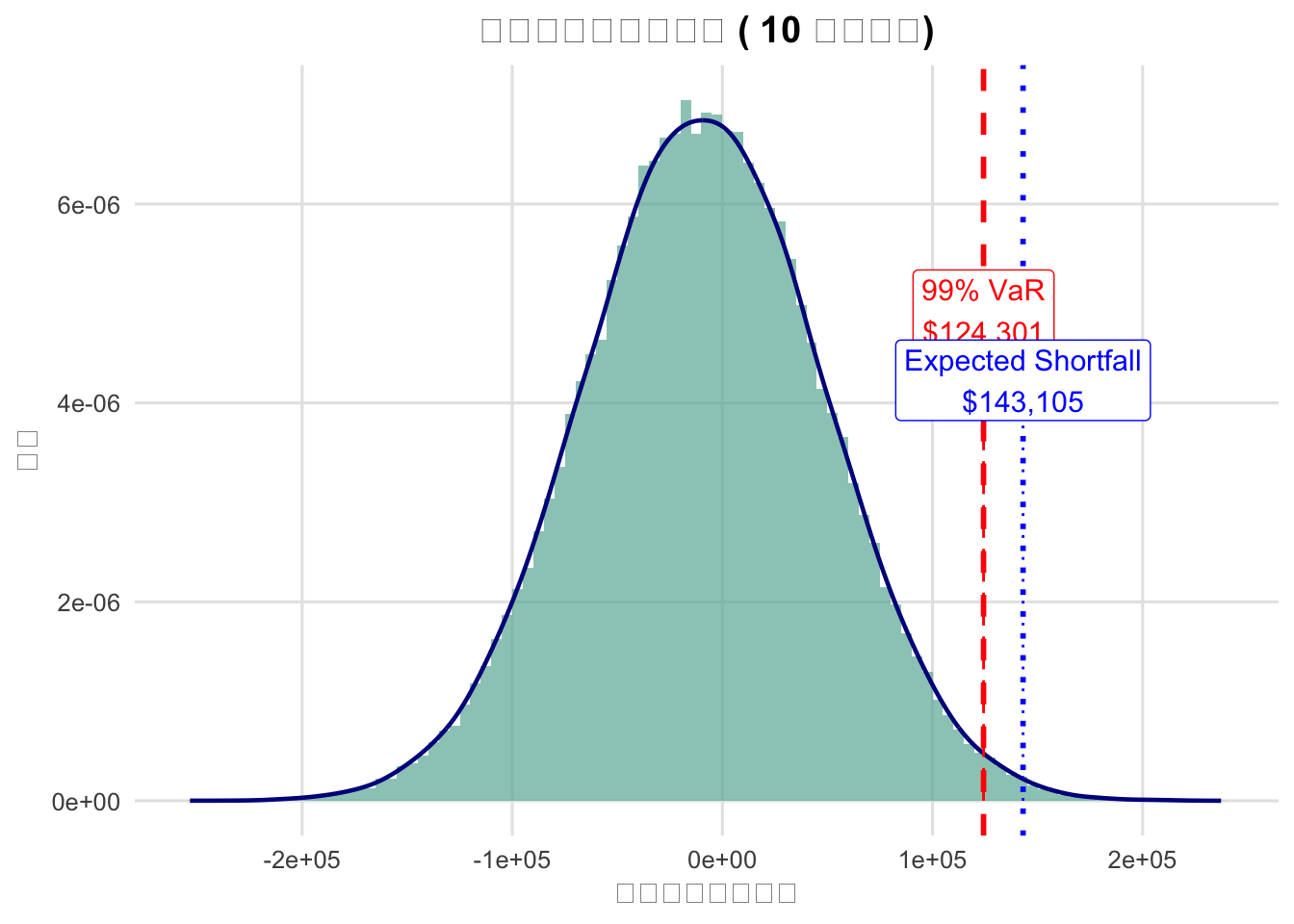
labs(title=paste("多资产组合损失分布 (",T_days,"天持有期)"),
x="损失金额(美元)", y="密度") +
theme_minimal(base_size=12) +
theme(
plot.title=element_text(hjust=0.5, face="bold"),
panel.grid.major=element_line(color="gray90"),
panel.grid.minor=element_blank()
)
## Warning: Using `size` aesthetic for lines was deprecated in ggplot2 3.4.0.
## ℹ Please use `linewidth` instead.
## This warning is displayed once every 8 hours.
## Call `lifecycle::last_lifecycle_warnings()` to see where this warning was
## generated.
# 动态计算标注位置
plot_data <- ggplot_build(loss_plot)
## Warning: The dot-dot notation (`..density..`) was deprecated in ggplot2 3.4.0.
## ℹ Please use `after_stat(density)` instead.
## This warning is displayed once every 8 hours.
## Call `lifecycle::last_lifecycle_warnings()` to see where this warning was
## generated.
max_density <- max(plot_data$data[[1]]$density)

loss_plot <- loss_plot +
  annotate("segment",
           x=VaR, xend=VaR,
           y=0, yend=0.65*max_density,
           color="red", linetype="dashed") +
  annotate("label",
           x=VaR, y=0.7*max_density,
           label=paste0(alpha*100, "% VaR\n$", format(round(VaR), big.mark=",")),
           color="red", fill="white", size=4) +
  annotate("segment",
           x=ES, xend=ES,
           y=0, yend=0.55*max_density,
           color="blue", linetype="dotted") +
  annotate("label",
           x=ES, y=0.6*max_density,
           label=paste0("Expected Shortfall\n$", format(round(ES), big.mark=",")),
           color="blue", fill="white", size=4)

print(loss_plot)
# ----------------------
# 结果输出
# ----------------------
cat(sprintf("\n【增强版蒙特卡洛模拟结果】(%d天持有期)\n", T_days))
##
## 【增强版蒙特卡洛模拟结果】(10天持有期)
cat("----------------------------------------\n")
## ----------------------------------------
cat(sprintf("▪ 投资组合规模: $%s\n", format(V0, big.mark=",")))
## ▪ 投资组合规模: $1e+06
cat(sprintf("▪ VaR(%d%%置信水平): $%s\n", alpha*100, format(round(VaR), big.mark=",")))
## ▪ VaR(99%置信水平): $124,519
cat(sprintf("▪ 预期损失(ES): $%s\n", format(round(ES), big.mark=",")))
## ▪ 预期损失(ES): $143,313
cat(sprintf("▪ 最大可能损失: $%s\n", format(round(max(losses)), big.mark=",")))
## ▪ 最大可能损失: $237,724
基于混合多元正态分布优化蒙特卡洛模拟法
混合多元正态分布可通过组合多个多元正态分布刻画不同市场状态下资产收益率的动态相关性和厚尾特征,适用于多资产组合的VaR计算。
在置信水平 \(\alpha\) 下,多元混合正态模型的分位数 \(Q_{\alpha}\) 满足以下等式:
$$
\sum_{i=1}^k \pi_i \cdot \Phi\left(Q_\alpha ,;, \mu_p^{(i)}, \sigma_p^{(i)}\right) = \alpha
$$
\(\pi_i\): 第\(i\)个混合成分的权重($\sum_{i=1}^k \pi_i = 1$);\(\mu_p^{(i)} = \mathbf{w}^\top \boldsymbol{\mu}_i\): 第\(i\)个成分的线性组合均值($\mathbf{w}$ 为资产权重向量,$\boldsymbol{\mu}_i$ 为成分均值向量);\(\sigma_p^{(i)} = \sqrt{\mathbf{w}^\top \boldsymbol{\Sigma}_i \mathbf{w}}\): 第\(i\)个成分的线性组合标准差($\boldsymbol{\Sigma}_i$ 为成分协方差矩阵);\(\Phi(\cdot)\): 标准单变量正态分布的累积分布函数(CDF)
# 加载包
library(quantmod)
library(mclust)
## Package 'mclust' version 6.1.1
## Type 'citation("mclust")' for citing this R package in publications.
library(MASS)
library(Matrix)
library(matrixcalc)
library(dplyr)
library(showtext)
## 载入需要的程序包:sysfonts
## 载入需要的程序包:showtextdb
library(ggplot2)
library(DescTools)
##
## 载入程序包:'DescTools'
## The following object is masked from 'package:mclust':
##
##     BrierScore
# 参数设置
symbols <- c("AAPL", "GOOG", "MSFT")
weights <- c(0.4, 0.3, 0.3)
portfolio_value <- 1e6
confidence_level <- 0.95

# 数据获取与处理
getSymbols(symbols, from = "2020-01-01", to = Sys.Date())
## [1] "AAPL" "GOOG" "MSFT"
prices <- do.call(merge, lapply(symbols, function(x) Cl(get(x))))
returns <- ROC(prices,type = "discrete") %>% na.omit() %>% as.matrix()

# 混合模型拟合与修正
set.seed(123)
mix_model <- Mclust(returns, G = 2)

# 提取并修正模型参数
weights_mix <- mix_model$parameters$pro
means_mix <- mix_model$parameters$mean

# 检查混合模型协方差参数维度
sigma_dim <- dim(mix_model$parameters$variance$sigma)
cat("Sigma参数维度:", sigma_dim, "\n")
## Sigma参数维度: 3 3 2
# 确认模型类型是否兼容
if (mix_model$modelName != "VVV") {
  warning("当前模型", mix_model$modelName,
          "可能使用共享协方差矩阵结构,需调整修正逻辑")
}


covs_mix <- lapply(1:mix_model$G, function(g) {
  # 提取第g个成分的协方差矩阵
  sigma <- mix_model$parameters$variance$sigma[,,g]

  # 验证矩阵维度
  if (!matrixcalc::is.square.matrix(sigma)) {
    stop(paste("成分", g, "协方差矩阵非正方形,维度:",
              paste(dim(sigma), collapse="x")))
  }

  # 特征值修正
  eig <- eigen(sigma)
  ev <- pmax(eig$values, 1e-6)
  sigma_corrected <- eig$vectors %*% diag(ev) %*% t(eig$vectors)
  as.matrix(nearPD(sigma_corrected)$mat)
})

# 增强型修正函数
robust_cov_fix <- function(sigma) {
  if (!is.matrix(sigma) || nrow(sigma) != ncol(sigma)) {
    sigma <- matrix(sigma, nrow=sqrt(length(sigma)))  # 向量转矩阵
  }

  # 添加对称性强制修正
  sigma <- 0.5 * (sigma + t(sigma))

  # 执行特征值修正
  eig <- eigen(sigma)
  ev <- pmax(eig$values, 1e-6)
  eig$vectors %*% diag(ev) %*% t(eig$vectors)
}

# 应用修正函数
covs_mix <- lapply(1:mix_model$G, function(g) {
  as.matrix(nearPD(
    robust_cov_fix(mix_model$parameters$variance$sigma[,,g])
  )$mat)
})

# 验证所有协方差矩阵性质
sapply(covs_mix, function(x) {
  c(dim=dim(x), isSquare=matrixcalc::is.square.matrix(x))
})  # 维度应统一为NxN
##          [,1] [,2]
## dim1        3    3
## dim2        3    3
## isSquare    1    1
# 检查正定性
sapply(covs_mix, matrixcalc::is.positive.definite)  # 应全为TRUE
## [1] TRUE TRUE
# 安全模拟函数
safe_mvrnorm <- function(n, mu, sigma) {
  sigma_fixed <- as.matrix(nearPD(sigma)$mat)
  MASS::mvrnorm(n, mu, sigma_fixed)
}

# 蒙特卡洛模拟
n_sim <- 10000
sim_returns <- matrix(0, nrow = n_sim, ncol = 3)

for (i in 1:n_sim) {
  component <- sample(1:length(weights_mix), 1, prob = weights_mix)
  sim_returns[i, ] <- safe_mvrnorm(1,
                                  means_mix[, component],
                                  covs_mix[[component]])
}

# 查看模拟结果摘要
summary(sim_returns)  # 不应有NA或极端值
##        V1                   V2                   V3
##  Min.   :-0.1235547   Min.   :-0.1244924   Min.   :-0.1164468
##  1st Qu.:-0.0101667   1st Qu.:-0.0104414   1st Qu.:-0.0098317
##  Median : 0.0012049   Median : 0.0009092   Median : 0.0006312
##  Mean   : 0.0009236   Mean   : 0.0006466   Mean   : 0.0007475
##  3rd Qu.: 0.0126020   3rd Qu.: 0.0120780   3rd Qu.: 0.0113348
##  Max.   : 0.1311838   Max.   : 0.1262479   Max.   : 0.1401261
# 计算VaR
portfolio_returns <- sim_returns %*% weights
portfolio_returns <- na.omit(portfolio_returns) # 移除缺失值
if (sd(portfolio_returns) < 1e-6) stop("收益波动率过低,无法生成有效分布")
# Winsorize处理极端值
portfolio_returns <- Winsorize(portfolio_returns)
losses <- -portfolio_value * portfolio_returns
# 计算VaR和ES
VaR <- quantile(losses, 1 - confidence_level)
ES <- mean(losses[losses <= VaR])
# 生成自适应breaks
br <- pretty(range(portfolio_returns), n = 100)
if (length(br) < 10) br <- seq(min(portfolio_returns), max(portfolio_returns), length.out=100)
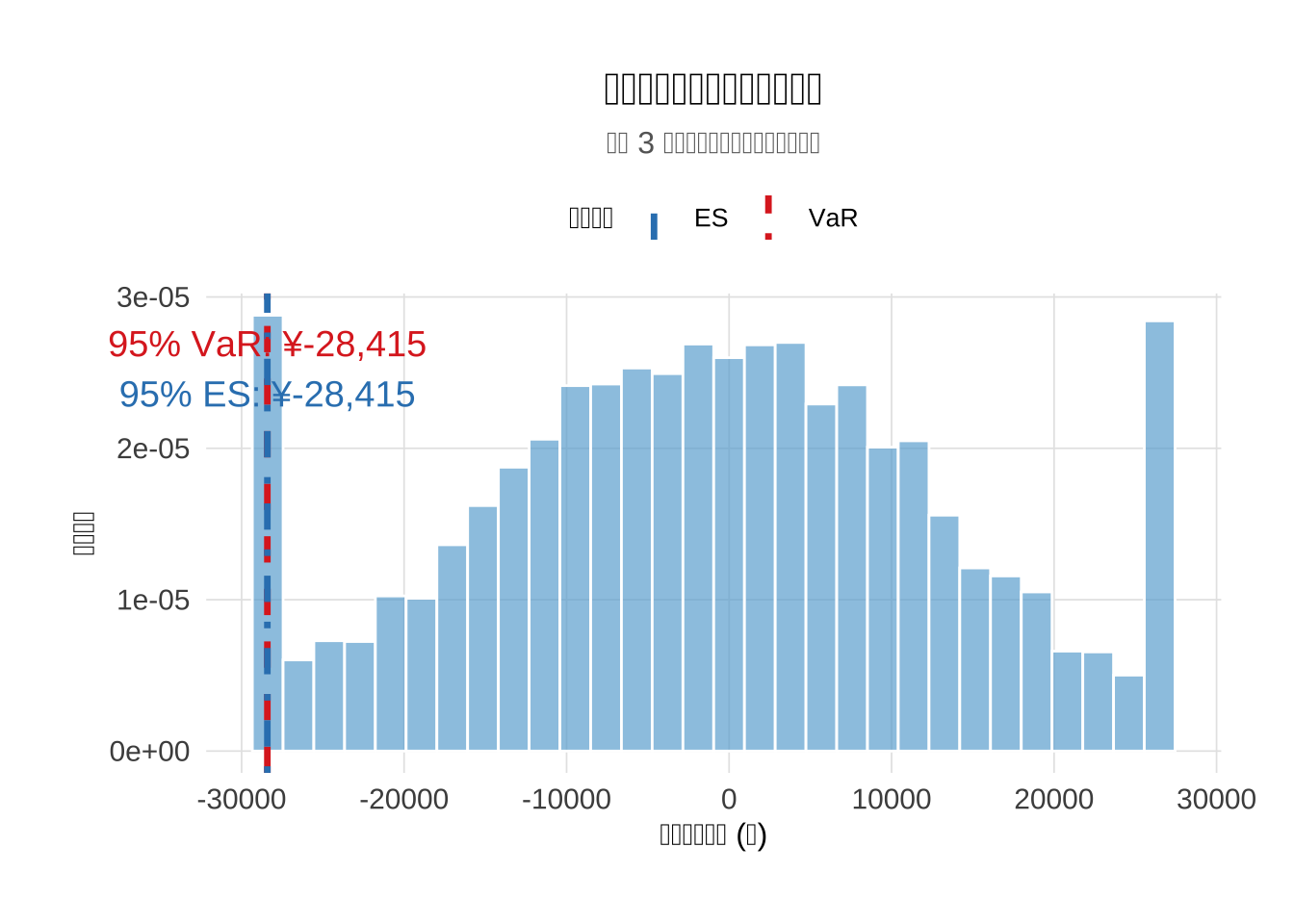
cat("95% VaR:", round(VaR, 2), "元\n")
## 95% VaR: -27728.82 元
cat("95% ES:",round(ES, 2),"元\n")
## 95% ES: -27729.96 元
# 验证VaR计算合理性
cat("VaR占组合比例:", round(VaR/portfolio_value*100, 2), "%\n")
## VaR占组合比例: -2.77 %
cat("ES占组合比例:", round(ES/portfolio_value*100,2),"%\n")
## ES占组合比例: -2.77 %
# 正常范围通常在1%-10%之间

showtext_auto()  # 启用中文字体支持

# 计算VaR和ES的标签文本
var_label <- paste0(confidence_level*100, "% VaR: ¥", format(round(VaR), big.mark = ","))
es_label <- paste0(confidence_level*100, "% ES: ¥", format(round(ES), big.mark = ","))

# 生成风险可视化图表
loss_plot <- ggplot(data.frame(losses), aes(x = losses)) +
  geom_histogram(aes(y = after_stat(density)),
                 fill = "#6baed6", alpha = 0.7, color = "white") +  # 优化填充色并添加边框
  geom_vline(aes(xintercept = VaR, color = "VaR"),
             linetype = "dashed", linewidth = 1.2) +
  geom_vline(aes(xintercept = ES, color = "ES"),
             linetype = "dotdash", linewidth = 1.2) +  # 添加ES线
  annotate("text", x = VaR, y = Inf, label = var_label,  # 使用annotate固定标签位置
           color = "#de2d26", vjust = 2.5, size = 5, family = "sans") +
  annotate("text", x = ES, y = Inf, label = es_label,
           color = "#3182bd", vjust = 4.5, size = 5, family = "sans") +
  scale_color_manual(name = "风险指标",
                     values = c("VaR" = "#de2d26", "ES" = "#3182bd"),
                     guide = guide_legend(override.aes = list(
                       linetype = c("dashed", "dotdash")))) +
  labs(title = "投资组合风险价值分布可视化",
       subtitle = paste("基于", length(symbols), "资产混合正态模型蒙特卡洛模拟"),
       x = "潜在损失金额 (元)", y = "概率密度") +
  theme_minimal(base_size = 14) +
  theme(
    text = element_text(family = "sans"),  # 确保中文字体显示
    plot.title = element_text(hjust = 0.5, face = "bold", size = 18),
    plot.subtitle = element_text(hjust = 0.5, color = "gray40", size = 12),
    axis.title = element_text(size = 12),
    axis.text = element_text(color = "gray30"),
    panel.grid.major = element_line(color = "grey90", linewidth = 0.3),
    panel.grid.minor = element_blank(),  # 移除次要网格线
    legend.position = "top",
    legend.title = element_text(size = 12),
    legend.text = element_text(size = 10),
    plot.margin = margin(1, 1, 1, 1, "cm")
  ) +
  coord_cartesian(clip = "off")  # 允许标签超出绘图区域

print(loss_plot)
## `stat_bin()` using `bins = 30`. Pick better value with `binwidth`.