方差-协方差法
方差-协方差法是一种基于资产收益率正态性假设的VaR计算方法。其核心思想是通过历史数据估计资产收益率的均值、方差和协方差矩阵,构建投资组合收益率的概率分布,继而计算VaR值。
具体流程可分为以下三步:
首先,计算资产收益率的协方差矩阵以衡量风险关联;其次,根据投资组合权重计算组合收益率的期望值和标准差;最后,在给定置信水平下,利用正态分布分位数确定VaR值。例如,在95%置信水平下,单日VaR可表示为组合市值的绝对值乘以其标准差再乘1.645(对应正态分布左尾5%分位数)。该方法计算效率高,但对非线性风险和非正态分布敏感。多日VaR可通过时间平方根法则调整,即单日VaR乘 \(\sqrt{T}\) 得到。
R代码实现
# 加载必要包
library(quantmod)
## 载入需要的程序包:xts
## 载入需要的程序包:zoo
##
## 载入程序包:'zoo'
## The following objects are masked from 'package:base':
##
##     as.Date, as.Date.numeric
## 载入需要的程序包:TTR
## Registered S3 method overwritten by 'quantmod':
##   method            from
##   as.zoo.data.frame zoo
library(PerformanceAnalytics)
##
## 载入程序包:'PerformanceAnalytics'
## The following object is masked from 'package:graphics':
##
##     legend
library(ggplot2)
library(dplyr)
##
## ######################### Warning from 'xts' package ##########################
## #                                                                             #
## # The dplyr lag() function breaks how base R's lag() function is supposed to  #
## # work, which breaks lag(my_xts). Calls to lag(my_xts) that you type or       #
## # source() into this session won't work correctly.                            #
## #                                                                             #
## # Use stats::lag() to make sure you're not using dplyr::lag(), or you can add #
## # conflictRules('dplyr', exclude = 'lag') to your .Rprofile to stop           #
## # dplyr from breaking base R's lag() function.                                #
## #                                                                             #
## # Code in packages is not affected. It's protected by R's namespace mechanism #
## # Set `options(xts.warn_dplyr_breaks_lag = FALSE)` to suppress this warning.  #
## #                                                                             #
## ###############################################################################
##
## 载入程序包:'dplyr'
## The following objects are masked from 'package:xts':
##
##     first, last
## The following objects are masked from 'package:stats':
##
##     filter, lag
## The following objects are masked from 'package:base':
##
##     intersect, setdiff, setequal, union
# 1. 下载股票数据(示例使用苹果、微软、亚马逊)
symbols <- c("AAPL", "MSFT", "AMZN")
getSymbols(symbols, src = "yahoo", from = "2022-01-01", to = Sys.Date())
## [1] "AAPL" "MSFT" "AMZN"
# 2. 提取收盘价并合并
prices <- merge(Cl(AAPL), Cl(MSFT), Cl(AMZN)) %>% na.omit()
colnames(prices) <- symbols
# 3. 计算对数收益率
returns <- na.omit(Return.calculate(prices, method = "log"))
# 4. 设定投资组合参数
weights <- c(0.3, 0.4, 0.3) # 组合权重
conf_level <- 0.95 # 置信水平
portfolio_value <- 1e6 # 组合价值(美元)
# 5. 计算协方差矩阵与组合标准差
cov_matrix <- cov(returns)
port_sd <- sqrt(t(weights) %*% cov_matrix %*% weights)
# 6. 计算单日VaR
var_1d <- abs(portfolio_value * qnorm(1 - conf_level) * port_sd)
# 7. 计算5日VaR(时间平方根法则)
var_5d <- var_1d * sqrt(5)
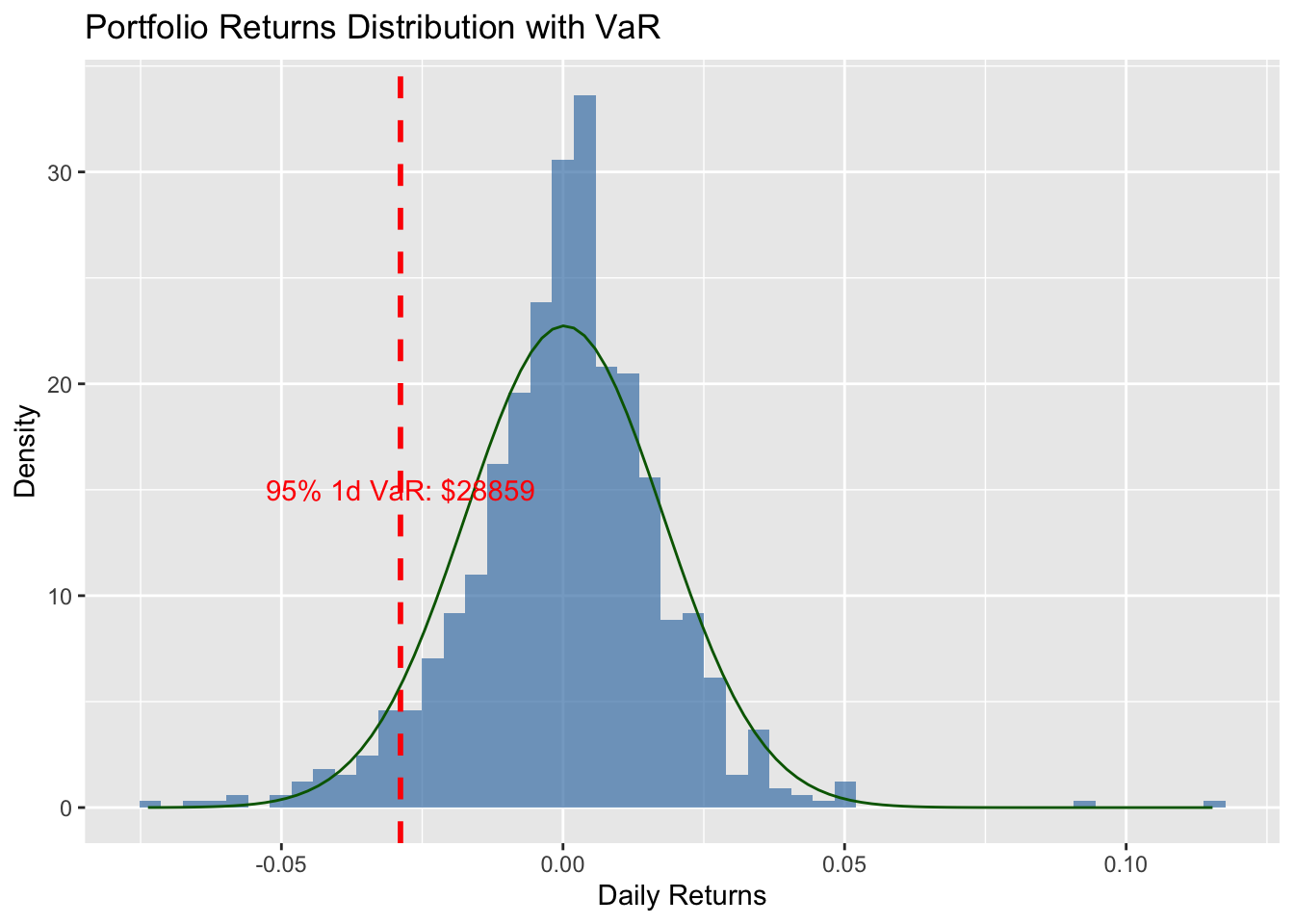
# 8. 可视化VaR分布
ggplot(data = data.frame(Returns = as.numeric(returns %*% weights)),
aes(x = Returns)) +
geom_histogram(aes(y = ..density..), bins = 50, fill = "steelblue", alpha = 0.7) +
geom_vline(xintercept = -var_1d/portfolio_value, color = "red",
linetype = "dashed", size = 1) +
stat_function(fun = dnorm, args = list(mean = mean(returns %*% weights),
sd = sd(returns %*% weights)), color = "darkgreen") +
labs(title = "Portfolio Returns Distribution with VaR",
x = "Daily Returns", y = "Density") +
annotate("text", x = -var_1d/portfolio_value, y = 15,
label = paste0("95% 1d VaR: $", round(var_1d)), color = "red")
## Warning: Using `size` aesthetic for lines was deprecated in ggplot2 3.4.0.
## ℹ Please use `linewidth` instead.
## This warning is displayed once every 8 hours.
## Call `lifecycle::last_lifecycle_warnings()` to see where this warning was
## generated.
## Warning: The dot-dot notation (`..density..`) was deprecated in ggplot2 3.4.0.
## ℹ Please use `after_stat(density)` instead.
## This warning is displayed once every 8 hours.
## Call `lifecycle::last_lifecycle_warnings()` to see where this warning was
## generated.
# 输出结果
cat("单日VaR(95%置信度):", round(var_1d), "美元\n")
## 单日VaR(95%置信度): 28894 美元
cat("5日VaR(95%置信度):", round(var_5d), "美元")
## 5日VaR(95%置信度): 64609 美元