需要用到的R包
xts和zoo是两个强大的处理时序对象的R包。xts包本身又相当于是一个加强版的zoo包。zoo包处理的对象是zoo,zoo对象与数据框(dataframe)类似,由行列构成。不同的是,zoo对象比数据框多了一个时间戳。
假设我们有一个zoo对象t,index(t)返回时间戳,也就是一个表示日期的向量。start(t)和end(t)可以查看zoo对象的起始值和末端值。
数据预处理
分四个步骤:
- 读入数据(data frame格式)
- 将日期转化为Date对象
- 将data frame数据转换为zoo对象
- 合并数据
相应的R代码:
library(quantmod) # 金融数据获取
## 载入需要的程序包:xts
## 载入需要的程序包:zoo
##
## 载入程序包:'zoo'
## The following objects are masked from 'package:base':
##
##     as.Date, as.Date.numeric
## 载入需要的程序包:TTR
## Registered S3 method overwritten by 'quantmod':
##   method            from
##   as.zoo.data.frame zoo
library(urca)       # 协整检验
library(ggplot2)    # 可视化

# 获取2010-2011年股票数据
getSymbols(c("AAPL","MSFT"))
## [1] "AAPL" "MSFT"
# 提取收盘价并转换为对数序列
aapl <- log(Ad(AAPL$AAPL.Adjusted))
msft <- log(Ad(MSFT$MSFT.Adjusted))

# 创建合并数据集
prices <- merge(aapl, msft)
colnames(prices) <- c("log_AAPL", "log_MSFT")

# 绘制对数价格趋势
ggplot(prices, aes(x=Index)) +
  geom_line(aes(y=log_AAPL, color="苹果")) +
  geom_line(aes(y=log_MSFT, color="微软")) +
  labs(title="苹果与微软对数收盘价序列", y="log(Price)", x="日期") +
  scale_color_manual(values=c("#FF6B6B", "#4ECDC4")) +
  theme_minimal(base_family = "PingFang SC")

平稳性检验
# 原始序列检验
# 苹果价格ADF检验
summary(ur.df(prices$log_AAPL, type="drift", lags=5)) #P-value大于0.05则序列不平稳
##
## ###############################################
## # Augmented Dickey-Fuller Test Unit Root Test #
## ###############################################
##
## Test regression drift
##
##
## Call:
## lm(formula = z.diff ~ z.lag.1 + 1 + z.diff.lag)
##
## Residuals:
##       Min        1Q    Median        3Q       Max
## -0.197346 -0.008942  0.000164  0.010330  0.141513
##
## Coefficients:
##               Estimate Std. Error t value Pr(>|t|)
## (Intercept)  0.0016271  0.0008139   1.999   0.0457 *
## z.lag.1     -0.0002047  0.0002258  -0.907   0.3646
## z.diff.lag1 -0.0321993  0.0147383  -2.185   0.0290 *
## z.diff.lag2 -0.0155993  0.0147150  -1.060   0.2892
## z.diff.lag3 -0.0090648  0.0147162  -0.616   0.5379
## z.diff.lag4  0.0250380  0.0147149   1.702   0.0889 .
## z.diff.lag5  0.0145020  0.0147113   0.986   0.3243
## ---
## Signif. codes:  0 '***' 0.001 '**' 0.01 '*' 0.05 '.' 0.1 ' ' 1
##
## Residual standard error: 0.01992 on 4600 degrees of freedom
## Multiple R-squared:  0.00234,	Adjusted R-squared:  0.001039
## F-statistic: 1.798 on 6 and 4600 DF,  p-value: 0.09538
##
##
## Value of test-statistic is: -0.9067 5.4705
##
## Critical values for test statistics:
##       1pct  5pct 10pct
## tau2 -3.43 -2.86 -2.57
## phi1  6.43  4.59  3.78
# 微软价格ADF检验
summary(ur.df(prices$log_MSFT, type="drift", lags=5))
##
## ###############################################
## # Augmented Dickey-Fuller Test Unit Root Test #
## ###############################################
##
## Test regression drift
##
##
## Call:
## lm(formula = z.diff ~ z.lag.1 + 1 + z.diff.lag)
##
## Residuals:
##       Min        1Q    Median        3Q       Max
## -0.148299 -0.008044  0.000121  0.008836  0.160776
##
## Coefficients:
##               Estimate Std. Error t value Pr(>|t|)
## (Intercept)  0.0001374  0.0010067   0.137  0.89142
## z.lag.1      0.0001571  0.0002344   0.670  0.50269
## z.diff.lag1 -0.1088675  0.0147498  -7.381 1.86e-13 ***
## z.diff.lag2 -0.0421217  0.0148530  -2.836  0.00459 **
## z.diff.lag3  0.0054135  0.0148661   0.364  0.71576
## z.diff.lag4 -0.0431566  0.0148530  -2.906  0.00368 **
## z.diff.lag5 -0.0185213  0.0147761  -1.253  0.21010
## ---
## Signif. codes:  0 '***' 0.001 '**' 0.01 '*' 0.05 '.' 0.1 ' ' 1
##
## Residual standard error: 0.01756 on 4600 degrees of freedom
## Multiple R-squared:  0.01478,	Adjusted R-squared:  0.0135
## F-statistic:  11.5 on 6 and 4600 DF,  p-value: 8.16e-13
##
##
## Value of test-statistic is: 0.6703 4.8403
##
## Critical values for test statistics:
##       1pct  5pct 10pct
## tau2 -3.43 -2.86 -2.57
## phi1  6.43  4.59  3.78
# 一阶差分平稳性验证
# 差分处理
diff_aapl <- diff(prices$log_AAPL)[-1]
diff_msft <- diff(prices$log_MSFT)[-1]

# 差分序列ADF检验
summary(ur.df(diff_aapl, type="none"))
##
## ###############################################
## # Augmented Dickey-Fuller Test Unit Root Test #
## ###############################################
##
## Test regression none
##
##
## Call:
## lm(formula = z.diff ~ z.lag.1 - 1 + z.diff.lag)
##
## Residuals:
##       Min        1Q    Median        3Q       Max
## -0.197910 -0.007903  0.001180  0.011336  0.140719
##
## Coefficients:
##            Estimate Std. Error t value Pr(>|t|)
## z.lag.1    -1.04076    0.02112 -49.286   <2e-16 ***
## z.diff.lag  0.01349    0.01473   0.916     0.36
## ---
## Signif. codes:  0 '***' 0.001 '**' 0.01 '*' 0.05 '.' 0.1 ' ' 1
##
## Residual standard error: 0.01999 on 4608 degrees of freedom
## Multiple R-squared:  0.5134,	Adjusted R-squared:  0.5131
## F-statistic:  2430 on 2 and 4608 DF,  p-value: < 2.2e-16
##
##
## Value of test-statistic is: -49.2864
##
## Critical values for test statistics:
##       1pct  5pct 10pct
## tau1 -2.58 -1.95 -1.62
summary(ur.df(diff_msft, type="none"))
##
## ###############################################
## # Augmented Dickey-Fuller Test Unit Root Test #
## ###############################################
##
## Test regression none
##
##
## Call:
## lm(formula = z.diff ~ z.lag.1 - 1 + z.diff.lag)
##
## Residuals:
##       Min        1Q    Median        3Q       Max
## -0.149197 -0.007368  0.000777  0.009507  0.165463
##
## Coefficients:
##            Estimate Std. Error t value Pr(>|t|)
## z.lag.1    -1.14697    0.02190 -52.367  < 2e-16 ***
## z.diff.lag  0.03991    0.01475   2.705  0.00685 **
## ---
## Signif. codes:  0 '***' 0.001 '**' 0.01 '*' 0.05 '.' 0.1 ' ' 1
##
## Residual standard error: 0.01758 on 4608 degrees of freedom
## Multiple R-squared:  0.5521,	Adjusted R-squared:  0.5519
## F-statistic:  2840 on 2 and 4608 DF,  p-value: < 2.2e-16
##
##
## Value of test-statistic is: -52.3667
##
## Critical values for test statistics:
##       1pct  5pct 10pct
## tau1 -2.58 -1.95 -1.62
协整检验
我们用Engle-Granger两步法进行协整检验。
# 第一步:构建回归模型
coint_model <- lm(log_AAPL ~ log_MSFT, data=prices)
summary(coint_model)  # 显示回归系数与R-squared
##
## Call:
## lm(formula = log_AAPL ~ log_MSFT, data = prices)
##
## Residuals:
##      Min       1Q   Median       3Q      Max
## -1.20523 -0.17828  0.03798  0.22297  0.77306
##
## Coefficients:
##              Estimate Std. Error t value Pr(>|t|)
## (Intercept) -1.343406   0.020650  -65.06   <2e-16 ***
## log_MSFT     1.131850   0.004805  235.54   <2e-16 ***
## ---
## Signif. codes:  0 '***' 0.001 '**' 0.01 '*' 0.05 '.' 0.1 ' ' 1
##
## Residual standard error: 0.3607 on 4611 degrees of freedom
## Multiple R-squared:  0.9233,	Adjusted R-squared:  0.9233
## F-statistic: 5.548e+04 on 1 and 4611 DF,  p-value: < 2.2e-16
# 提取残差序列
residuals <- residuals(coint_model)

# 第二步:残差平稳性检验
adf_test <- ur.df(residuals, type="none", lags=5)
print(adf_test@teststat)    # ADF统计量
##                tau1
## statistic -2.893062
print(adf_test@cval) # 临界值
##       1pct  5pct 10pct
## tau1 -2.58 -1.95 -1.62
ADF统计量为-2.893062,小于1%置信水平对应的临界值-2.58,故拒绝原假设,说明残差序列平稳,两股票存在协整关系。
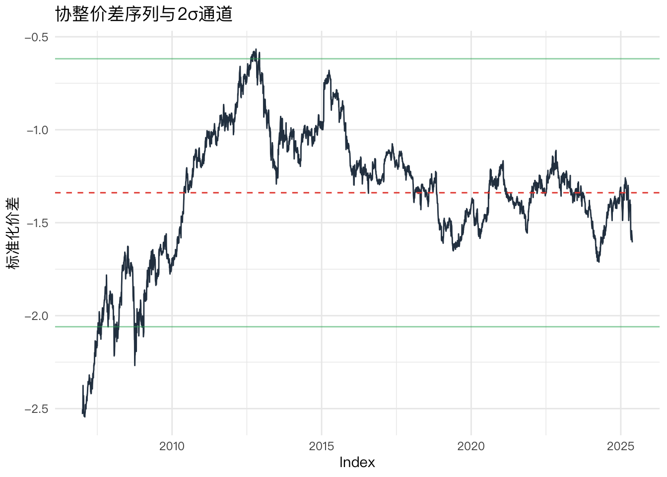
对协整关系进行可视化
# 计算价差序列
spread <- prices$log_AAPL - coint_model$coefficients[2] * prices$log_MSFT

# 绘制价差通道
ggplot(spread, aes(x=Index)) +
  geom_line(aes(y=spread), color="#2C3E50") +
  geom_hline(yintercept=mean(spread), linetype="dashed", color="#E74C3C") +
  geom_hline(yintercept=mean(spread)+2*sd(spread), color="#27AE60", alpha=0.5) +
  geom_hline(yintercept=mean(spread)-2*sd(spread), color="#27AE60", alpha=0.5) +
  labs(title="协整价差序列与2σ通道", y="标准化价差")+
  theme_minimal(base_family = "PingFang SC")
## Don't know how to automatically pick scale for object of type <xts/zoo>.
## Defaulting to continuous.