理论基础概述
在金融风险管理领域,风险价值(VaR)是一种广泛使用的风险度量工具,它衡量在一定置信水平下,某一金融资产或投资组合在未来特定时期内可能遭受的最大损失。然而,VaR 存在一些局限性,主要体现在以下几个方面:
- 缺乏次可加性:在某些情况下,投资组合的 VaR 可能大于其各组成部分 VaR 之和,这与分散投资降低风险的直觉相悖。
- 对尾部风险的刻画不足:VaR 只关注损失分布的分位数点,而不考虑超过该点的损失程度。
- 不满足一致性风险度量的要求:VaR 不满足一致性风险度量公理中的次可加性、正齐次性、单调性和平移不变性。
为了克服 VaR 的这些局限性,条件风险价值(CVaR)和预期短缺(ES)作为更高级的风险度量方法被提出。CVaR 与 ES 的基本概念条件风险价值(Conditional Value at Risk, CVaR),也称为平均短缺(Average Shortfall, AS)或预期短缺(Expected Shortfall, ES),是指在给定置信水平下,超过 VaR 的损失的期望值。
它不仅考虑了损失超过 VaR 的概率,还考虑了超过部分的大小,因此能更全面地反映尾部风险。
数学公式解析
VaR 的数学定义
对于给定的投资组合收益率 R 和置信水平 \(\alpha\),VaR 可以定义为:
\[ \text{VaR}_\alpha = -\inf \{ x \in \mathbb{R} : F_R(x) \geq \alpha \} \]
其中,\(F_R(x)\) 是收益率 \(R\) 的累积分布函数。
在实际应用中,VaR 通常表示为:
\[ P(R \leq -\text{VaR}_\alpha) = 1 - \alpha \]
CVaR/ES 的数学定义
CVaR/ES 在置信水平 \(\alpha\) 下的定义为:
\[ \text{CVaR}_\alpha = \text{ES}_\alpha = \mathbb{E}[-R | R \leq -\text{VaR}_\alpha] \]
当收益率分布连续时,CVaR/ES 可以表示为:
\[ \text{ES}_\alpha = \frac{1}{1-\alpha} \int_{0}^{1-\alpha} \text{VaR}_p \, dp \]
这个公式表明,ES 是所有低于 \(\alpha\) 置信水平的 VaR 的平均值。
R 语言实现示例
下面通过 R 语言实现基于纳斯达克数据的 VaR、CVaR 和 ES 计算,使用 quantmod 包获取数据,并对比不同 R 包的计算方法。
使用 quantmod 获取数据
# 加载必要的包
library(quantmod)
library(PerformanceAnalytics)
library(xts)
library(tibble)
library(dplyr)
library(ggplot2)
library(showtext)  # 用于设置中文字体

# 设置中文字体
font_add("SimHei", "SimHei.ttf")  # 如果字体已安装
# 如果字体未安装,可以尝试系统字体路径
# font_add("SimHei", "/path/to/SimHei.ttf")  # Linux/Mac
# font_add("SimHei", "C:/Windows/Fonts/simhei.ttf")  # Windows

showtext_auto()  # 自动启用showtext

# 获取纳斯达克综合指数数据
getSymbols("^IXIC", from = "2020-01-01", to = Sys.Date())
## [1] "IXIC"# 计算日对数收益率
returns <- diff(log(Cl(IXIC)))
returns <- na.omit(returns)
# 设置置信水平
alpha <- 0.95
risk_results <- list()使用不同 R 包计算 ES/CVaR
PerformanceAnalytics 包
# 使用PerformanceAnalytics包计算ES

VaR_historical <- PerformanceAnalytics::VaR(returns, p = alpha , method = "historical")
VaR_gaussian <- PerformanceAnalytics::VaR(returns, p = alpha , method = "gaussian")
es_historical <- PerformanceAnalytics::ES(returns, p = alpha, method = "historical")
es_gaussian <- PerformanceAnalytics::ES(returns, p = alpha, method = "gaussian")

cat("PerformanceAnalytics包计算结果:\n")
## PerformanceAnalytics包计算结果:cat("历史模拟法 VaR:", round(VaR_historical * 100, 2), "%\n")## 历史模拟法 VaR: -2.58 %cat("正态分布假设 VaR:", round(VaR_gaussian * 100, 2), "%\n")## 正态分布假设 VaR: -2.64 %cat("历史模拟法 ES:", round(es_historical * 100, 2), "%\n")## 历史模拟法 ES: -3.91 %cat("正态分布假设 ES:", round(es_gaussian * 100, 2), "%\n")## 正态分布假设 ES: -3.32 %risk_results[["performance"]] <- list(
VaR_historical = VaR_historical,
VaR_gaussian = VaR_gaussian,
es_historical = es_historical,
es_gaussian = es_gaussian
)fGarch 包
# 使用fGarch包计算ES
library(fGarch)
# 拟合GARCH模型并预测
garch_model <- garchFit(~garch(1,1), data = returns, trace = FALSE)
forecast <- predict(garch_model, n.ahead = 1)
es_garch <- tail(fGarch::ES(garch_model), n = 1)
var_garch <- tail(fGarch::VaR(garch_model), n = 1)
cat("\nfGarch包计算结果:\n")
##
## fGarch包计算结果:cat("GARCH模型预测 VaR:", round(var_garch * 100, 2), "%\n")## GARCH模型预测 VaR: 1.47 %cat("GARCH模型预测 ES:", round(es_garch * 100, 2), "%\n")## GARCH模型预测 ES: 1.86 %risk_results[["fgarch"]] <- list(
var_garch = var_garch,
es_garch = es_garch
)cvar包(针对连续分布的VaR/ES计算)
if (!require("cvar")) install.packages("cvar")## Loading required package: cvar##
## Attaching package: 'cvar'## The following objects are masked from 'package:PerformanceAnalytics':
##
## ES, VaRlibrary(cvar)
# 标准正态分布计算
gaussian_es <- list(
qf = cvar::ES(qnorm, dist.type = "qf"), # 使用分位数函数
cdf = cvar::ES(pnorm, dist.type = "cdf") # 使用累积分布函数
)
# t分布计算(df=4)
t_dist_es <- list(
qf = cvar::ES(qt, dist.type = "qf", df = 4),
cdf = cvar::ES(pt, dist.type = "cdf", df = 4)
)
risk_results[["cvar"]] <- list(
gaussian_es = gaussian_es,
t_dist_es = t_dist_es
)- rugarch 包
# 加载必要的包
library(rugarch)
## Loading required package: parallellibrary(xts) # 处理时间序列数据
# 定义GARCH模型(使用偏态t分布)
spec <- ugarchspec(
variance.model = list(model = "sGARCH", garchOrder = c(1, 1)),
mean.model = list(armaOrder = c(0, 0), include.mean = TRUE),
distribution.model = "sstd" # 偏态t分布
)
# 拟合模型
fit <- ugarchfit(spec, data = returns, solver = "hybrid")
# 使用固定参数重新过滤数据
spec2 <- spec
setfixed(spec2) <- as.list(coef(fit))
filt <- ugarchfilter(spec2, data = returns, n.old = 1000)
# 提取拟合值和波动率
mu <- fitted(filt) # 条件均值
sigma_t <- sigma(filt) # 条件波动率
# 获取分布参数
skew <- coef(fit)["skew"]
shape <- coef(fit)["shape"]
# 计算VaR (使用向量化方法)
p <- 0.05 # 置信水平(1-95%)
VaR <- mu + sigma_t * qdist("sstd", p = p, mu = 0, sigma = 1, skew = skew, shape = shape)
# 计算ES (使用数值积分)
es_integrand <- function(x) {
qdist("sstd", p = x, mu = 0, sigma = 1, skew = skew, shape = shape)
}
# 向量化积分计算(对每个时间点单独计算ES)
ES <- numeric(length(returns))
for (i in 1:length(returns)) {
int_result <- integrate(es_integrand, lower = 0, upper = p, subdivisions = 1000)
ES[i] <- mu[i] + sigma_t[i] * int_result$value / p
}
# 确保所有向量长度一致(处理可能的长度差异)
min_len <- min(length(returns), length(VaR), length(ES))
actual <- as.numeric(tail(returns, min_len))
VaR <- tail(as.numeric(tail(VaR, min_len)),1)
ES <- tail(as.numeric(tail(ES, min_len)),1)
risk_results[["rugarch"]] <- list(
VaR = VaR,
ES = ES
)- gets包(基于ARX模型的条件风险度量)
# 加载必要的包
library(gets)
##
## Attaching package: 'gets'## The following objects are masked from 'package:cvar':
##
## ES, VaR## The following objects are masked from 'package:fGarch':
##
## ES, VaR## The following objects are masked from 'package:PerformanceAnalytics':
##
## ES, VaRreturns <- diff(log(Cl(IXIC)))
returns <- as.vector(na.omit(returns)) # 强制转换为普通向量
# 设置置信水平
alpha <- 0.95
# 构建ARX模型(滞后1阶)
# 使用普通向量而非xts对象
arx_model <- arx(returns, mc=TRUE, ar=1) # 直接使用向量格式
# 计算VaR和ES
risk_results[["gets"]] <- list(
VaR = quantile(arx_model$residuals, probs=1-alpha),
ES = mean(arx_model$residuals[arx_model$residuals <= quantile(arx_model$residuals, probs=1-alpha)])
)
# 打印结果
cat("ARX模型风险度量结果:\n")## ARX模型风险度量结果:cat("VaR (", alpha*100, "%):", round(risk_results[["gets"]]$VaR*100, 2), "%\n")## VaR ( 95 %): -2.64 %cat("ES (", alpha*100, "%):", round(risk_results[["gets"]]$ES*100, 2), "%\n")## ES ( 95 %): -3.93 %- MSGARCH包(贝叶斯方法的风险预测)
if (!require("MSGARCH")) install.packages("MSGARCH")## Loading required package: MSGARCHlibrary(MSGARCH)
spec_msgarch <- CreateSpec()
fit_msgarch <- FitML(spec_msgarch, data = returns)
risk_msgarch <- Risk(fit_msgarch, n.ahead = 1, level = alpha)
risk_results[["MSGARCH"]] <- list(
VaR = as.numeric(risk_msgarch$VaR),
ES = as.numeric(risk_msgarch$ES)
)- VaRES包(多种参数分布的风险度量)
if (!require("VaRES")) install.packages("VaRES")## Loading required package: VaRESlibrary(VaRES)
returns <- diff(log(Cl(IXIC)))
returns <- as.vector(na.omit(returns)) # 强制转换为普通向量
# 手动计算 VaR 和 ES(假设 df = 4)
df <- 4
alpha <- 0.05 # 95% 置信水平
# 计算 t 分布的 VaR
VaR_t <- -quantile(rt(n = 1e6, df = df), probs = alpha) * sd(returns)
# 计算 t 分布的 ES(解析解)
ES_t <- (dt(qt(alpha, df = df), df = df) / alpha) *
((df + qt(alpha, df = df)^2) / (df - 2)) *
sd(returns)
risk_results[["VaRES"]] <- list(VaR = VaR_t, ES = ES_t)结果对比与可视化
# 从risk_results中提取各方法的VaR和ES(统一格式:保留数值,处理符号)
returns_vec <- as.vector(returns)  # 转换为向量用于部分模型

results <- tibble(
  方法 = c(
    "历史模拟法",
    "正态分布假设",
    "GARCH(fGarch)",
    "GARCH(rugarch)",
    "MSGARCH",
    "ARX模型(gets)",
    "t分布(VaRES)"
  ),
  # 提取VaR(统一为损失幅度,取绝对值或修正符号)
  VaR = c(
    as.numeric(risk_results$performance$VaR_historical) %>% abs(),  # 历史模拟法
    as.numeric(risk_results$performance$VaR_gaussian) %>% abs(),   # 正态分布
    as.numeric(risk_results$fgarch$var_garch),                     # fGarch
    as.numeric(risk_results$rugarch$VaR) %>% abs(),                # rugarch
    as.numeric(risk_results$MSGARCH$VaR[1]) %>% abs(),             # MSGARCH(取第一个结果)
    as.numeric(risk_results$gets$VaR) %>% abs(),                   # ARX模型
    as.numeric(risk_results$VaRES$VaR)                             # VaRES包
  ),
  # 提取ES(统一为损失幅度,取绝对值或修正符号)
  ES = c(
    as.numeric(risk_results$performance$es_historical) %>% abs(),  # 历史模拟法
    as.numeric(risk_results$performance$es_gaussian) %>% abs(),   # 正态分布
    as.numeric(risk_results$fgarch$es_garch),                     # fGarch
    as.numeric(risk_results$rugarch$ES) %>% abs(),                # rugarch
    as.numeric(risk_results$MSGARCH$ES[1]) %>% abs(),             # MSGARCH(取第一个结果)
    as.numeric(risk_results$gets$ES) %>% abs(),                   # ARX模型
    as.numeric(risk_results$VaRES$ES)                             # VaRES包
  )
)

# 转换为百分比(乘以100)
results <- results %>%
  mutate(
    VaR_pct = VaR * 100,
    ES_pct = ES * 100
  )


# 不同方法的ES对比图
ggplot(results, aes(x = 方法, y = ES_pct, fill = 方法)) +
  geom_col(width = 0.7, show.legend = FALSE) +  # 柱状图,不显示图例
  geom_text(
    aes(label = sprintf("%.2f%%", ES_pct)),  # 显示百分比标签
    vjust = -0.5, size = 4, family = "SimHei"
  ) +
  labs(
    title = "不同方法计算的预期损失(ES)对比",
    x = "风险度量方法",
    y = "ES(%)",
    caption = "数据来源:纳斯达克指数(2020-2025)日对数收益率"
  ) +
  ylim(0, max(results$ES_pct) * 1.2) +  # 调整y轴范围,避免标签超出
  theme_minimal(base_family = "SimHei") +
  theme(
    plot.title = element_text(hjust = 0.5, face = "bold", size = 14),
    axis.text.x = element_text(angle = 45, hjust = 1, size = 10),
    plot.caption = element_text(hjust = 0, size = 8, color = "gray50")
  )
# 不同方法的VaR对比图
ggplot(results, aes(x = 方法, y = VaR_pct, fill = 方法)) +
  geom_col(width = 0.7, show.legend = FALSE) +
  geom_text(
    aes(label = sprintf("%.2f%%", VaR_pct)),
    vjust = -0.5, size = 4, family = "SimHei"
  ) +
  labs(
    title = "不同方法计算的风险价值(VaR)对比",
    x = "风险度量方法",
    y = "VaR(%)",
    caption = "数据来源:纳斯达克指数(2020-2025)日对数收益率"
  ) +
  ylim(0, max(results$VaR_pct) * 1.2) +
  theme_minimal(base_family = "SimHei") +
  theme(
    plot.title = element_text(hjust = 0.5, face = "bold", size = 14),
    axis.text.x = element_text(angle = 45, hjust = 1, size = 10),
    plot.caption = element_text(hjust = 0, size = 8, color = "gray50")
  )
# 收益率分布与ES标记
# 绘制收益率直方图,并标记历史模拟法ES
p <- ggplot(data = tibble(returns = returns_vec), aes(x = returns)) +
  geom_histogram(
    aes(y = after_stat(density)),  # 密度直方图
    bins = 50, fill = "lightblue", color = "white"
  ) +
  # 添加核密度曲线
  geom_density(color = "darkblue", linewidth = 0.8) +
  # 标记历史模拟法ES(取绝对值对应的收益率位置)
  geom_vline(
    xintercept = -results$ES[results$方法 == "历史模拟法"] / 100,  # 转换为收益率(负值表示损失)
    color = "red", linewidth = 1.2, linetype = "dashed"
  ) +
  annotate(
    "text", x = -results$ES[results$方法 == "历史模拟法"] / 100, y = 5,
    label = sprintf("历史模拟法ES: %.2f%%", results$ES[results$方法 == "历史模拟法"]),
    color = "red", hjust = 1.1, family = "SimHei"
  ) +
  labs(
    title = "纳斯达克指数日对数收益率分布",
    x = "日对数收益率",
    y = "密度"
  ) +
  theme_minimal(base_family = "SimHei") +
  theme(
    plot.title = element_text(hjust = 0.5, face = "bold")
  )
print(p)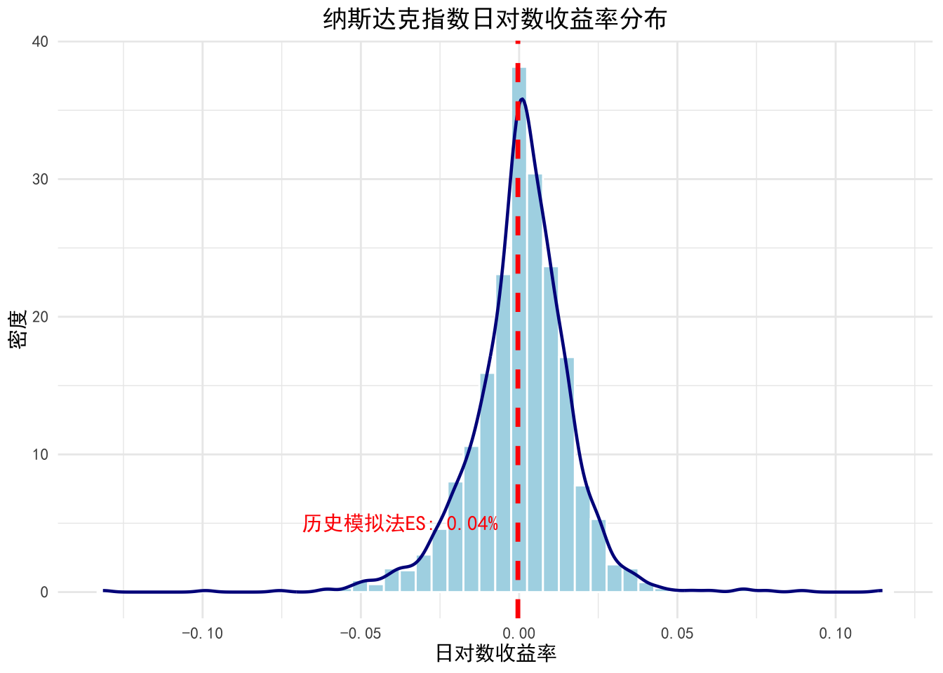
# ----------------------
# 输出数值结果
# ----------------------
cat("各方法风险度量结果(百分比):\n")
## 各方法风险度量结果(百分比):results %>%
select(方法, VaR_pct, ES_pct) %>%
rename(
"风险度量方法" = 方法,
"VaR(%)" = VaR_pct,
"ES(%)" = ES_pct
) %>%
print(n = Inf)## # A tibble: 7 × 3
## 风险度量方法 `VaR(%)` `ES(%)`
## <chr> <dbl> <dbl>
## 1 历史模拟法 2.58 3.91
## 2 正态分布假设 2.64 3.32
## 3 GARCH(fGarch) 1.47 1.86
## 4 GARCH(rugarch) 1.48 2.07
## 5 MSGARCH 2.25 2.73
## 6 ARX模型(gets) 2.64 3.93
## 7 t分布(VaRES) 3.47 7.87结论CVaR 和 ES 作为 VaR 的补充工具,能够更全面地度量金融风险,尤其是在处理尾部风险时表现更为出色。通过结合使用 VaR、CVaR 和 ES,风险管理者可以获得更完整的风险图景,从而做出更明智的风险管理决策。在实际应用中,应根据投资组合的特性和市场环境选择合适的风险度量方法。
不同 R 包提供了多种计算 ES/CVaR 的方法,各有特点:PerformanceAnalytics:简单易用,支持多种分布假设RiskPortfolios:专注投资组合风险分析fGarch/rugarch:适合结合 GARCH 模型处理时变波动率ExpectedShortfall:提供 ES 回测功能建议结合数据特性(如是否存在厚尾、波动聚类等)选择合适的模型,并对比不同方法的结果以确保对极端风险的充分考虑。