引言
XGBoost(eXtreme Gradient Boosting)是一种高效的梯度提升算法,在数据科学和机器学习领域广泛应用,尤其擅长处理结构化数据的回归和分类问题。以下从数学原理、发展历程、使用方法和竞争算法四个方面进行详细介绍:
一、数学原理
XGBoost 是梯度提升框架(Gradient Boosting)的优化实现,其核心思想是迭代地训练多个弱学习器(通常是决策树),并将它们组合成一个强学习器。
具体数学原理如下:
1.目标函数
XGBoost 的目标函数由两部分组成:
损失函数:衡量模型预测值与真实值之间的误差(如均方误差 MSE、对数损失 log loss 等)。 正则化项:控制模型复杂度,防止过拟合,包括树的数量、深度、叶子节点数等。
目标函数表达式:
\[ \text{Obj}(\theta) = \sum_{i=1}^n L(y_i, \hat{y}_i) + \sum_{k=1}^K \Omega(f_k) \]
其中:
- \(L(y_i, \hat{y}_i)\) 是样本 \(i\) 的损失函数,\(\hat{y}_i\) 是预测值,\(y_i\) 是真实值。
- \(\Omega(f_k)\) 是第 \(k\) 棵树的正则化项,通常包括树的复杂度(如叶子节点数、叶子节点权重的 L2 正则化)。
2.梯度提升迭代
XGBoost 通过迭代方式逐步优化目标函数:
初始化模型为常数预测: \(\hat{y}_i^{(0)} = \text{argmin}_c \sum_{i=1}^n L(y_i, c)\) 。
对于每一轮迭代 \(t\) :
- 计算损失函数关于当前预测值的梯度(一阶导数)和海森矩阵(二阶导数)。
- 训练一棵新的决策树 \(f_t\) ,拟合这些梯度(即预测梯度方向)。
- 更新预测值:\(\hat{y}_i^{(t)} = \hat{y}_i^{(t-1)} + \eta f_t(x_i)\) ,其中 \(\eta\) 是学习率(控制每次迭代的步长)。
3.决策树优化
XGBoost 在构建决策树时采用了以下优化策略:
- 精确贪心算法:通过枚举所有特征的所有可能分割点,找到最优分割。
- 近似算法:对于大规模数据,使用直方图近似快速找到分割点。
- 缺失值处理:自动学习缺失值的最优分裂方向。
- 正则化剪枝:通过正则化项控制树的复杂度,避免过拟合。
二、发展历程
2014 年:陈天奇(Tianqi Chen)在华盛顿大学读博期间开发了 XGBoost 的原型,最初作为研究项目用于解决大规模机器学习问题。
2015 年:XGBoost 作为开源项目发布,因其在 Kaggle 竞赛中的优异表现迅速走红,成为数据科学领域的主流算法之一。
2016 年:陈天奇加入微软,带领团队进一步优化 XGBoost,支持分布式计算和云计算平台。
2017 年至今:XGBoost 持续更新,增加了更多功能(如 DART、GPU 加速、特征重要性分析等),并被集成到多种编程语言和工具中(如 Python、R、Scala 等)。
三、如何使用
我们将用联邦基金有效利率和失业率为输入参数,按照 xgboost 模型对纳斯达克 100 指数月度数据进行建模。
# 加载必要的R包
library(tidyquant)      # 获取数据
## Registered S3 method overwritten by 'quantmod':
## method from
## as.zoo.data.frame zoo## ── Attaching core tidyquant packages ────────────────── tidyquant 1.0.11.9000 ──
## ✔ PerformanceAnalytics 2.0.8 ✔ TTR 0.24.4
## ✔ quantmod 0.4.28 ✔ xts 0.14.1
## ── Conflicts ────────────────────────────────────────── tidyquant_conflicts() ──
## ✖ zoo::as.Date() masks base::as.Date()
## ✖ zoo::as.Date.numeric() masks base::as.Date.numeric()
## ✖ PerformanceAnalytics::legend() masks graphics::legend()
## ✖ quantmod::summary() masks base::summary()
## ℹ Use the conflicted package (<http://conflicted.r-lib.org/>) to force all conflicts to become errorslibrary(tidyverse) # 数据处理与可视化的核心包集合## ── Attaching core tidyverse packages ──────────────────────── tidyverse 2.0.0 ──
## ✔ dplyr 1.1.4 ✔ readr 2.1.5
## ✔ forcats 1.0.0 ✔ stringr 1.5.1
## ✔ ggplot2 3.5.2 ✔ tibble 3.3.0
## ✔ lubridate 1.9.4 ✔ tidyr 1.3.1
## ✔ purrr 1.0.4
## ── Conflicts ────────────────────────────────────────── tidyverse_conflicts() ──
## ✖ dplyr::filter() masks stats::filter()
## ✖ dplyr::first() masks xts::first()
## ✖ dplyr::lag() masks stats::lag()
## ✖ dplyr::last() masks xts::last()
## ℹ Use the conflicted package (<http://conflicted.r-lib.org/>) to force all conflicts to become errorslibrary(tidymodels) # 机器学习建模框架## ── Attaching packages ────────────────────────────────────── tidymodels 1.3.0 ──
## ✔ broom 1.0.8 ✔ rsample 1.3.0
## ✔ dials 1.4.0 ✔ tune 1.3.0
## ✔ infer 1.0.9 ✔ workflows 1.2.0
## ✔ modeldata 1.4.0 ✔ workflowsets 1.1.1
## ✔ parsnip 1.3.2 ✔ yardstick 1.3.2
## ✔ recipes 1.3.1
## ── Conflicts ───────────────────────────────────────── tidymodels_conflicts() ──
## ✖ scales::discard() masks purrr::discard()
## ✖ dplyr::filter() masks stats::filter()
## ✖ dplyr::first() masks xts::first()
## ✖ recipes::fixed() masks stringr::fixed()
## ✖ dplyr::lag() masks stats::lag()
## ✖ dplyr::last() masks xts::last()
## ✖ dials::momentum() masks TTR::momentum()
## ✖ yardstick::spec() masks readr::spec()
## ✖ recipes::step() masks stats::step()library(modeltime) # 时间序列建模与预测##
## Attaching package: 'modeltime'
##
## The following object is masked from 'package:TTR':
##
## growthlibrary(timetk) # 时间序列数据处理工具##
## Attaching package: 'timetk'
##
## The following object is masked from 'package:tidyquant':
##
## FANG# 获取失业率数据 (UNRATE)
df_unrate <-
tq_get("UNRATE", get = "economic.data") %>%
select(date, unrate = price) # 重命名价格列为unrate
# 获取联邦基金有效利率数据 (FEDFUNDS)
df_fedfunds <-
tq_get("FEDFUNDS", get = "economic.data") %>%
select(date, fedfunds = price) # 重命名价格列为fedfunds
# 获取纳斯达克100指数数据
df_nasdaq <-
tq_get("^NDX") %>%
tq_transmute(select = close, # 选择收盘价
mutate_fun = to.monthly, # 转换为月度数据
col_rename = "nasdaq") %>% # 重命名列
mutate(date = as.Date(date)) # 确保日期格式正确
# 合并三个数据集
df_merged <-
df_unrate %>%
left_join(df_fedfunds) %>%
left_join(df_nasdaq) %>%
drop_na() # 删除包含缺失值的行## Joining with `by = join_by(date)`
## Joining with `by = join_by(date)`# 时间序列数据分割
splits <-
time_series_split(
df_merged,
assess = "1 year", # 测试集为1年数据
cumulative = TRUE # 训练集包含所有历史数据
)## Using date_var: datedf_train <- training(splits) # 提取训练集
df_test <- testing(splits) # 提取测试集
# 创建机器学习预处理配方
recipe_ml <-
recipe(nasdaq ~ ., df_train) %>% # 以nasdaq为目标变量
step_date(date, features = "month", ordinal = FALSE) %>% # 从日期提取月份特征
step_dummy(all_nominal_predictors(), one_hot = TRUE) %>% # 将分类变量转为虚拟变量
step_mutate(date_num = as.numeric(date)) %>% # 将日期转换为数值型
step_normalize(all_numeric_predictors()) %>% # 标准化数值预测变量
step_rm(date) # 移除原始日期列
# 定义XGBoost提升树模型规格,设置超参数为待调优
mod_spec <-
boost_tree(trees = tune(), # 树的数量
min_n = tune(), # 节点最小样本量
tree_depth = tune(), # 树的最大深度
learn_rate = tune()) %>% # 学习率
set_engine("xgboost") %>% # 使用xgboost引擎
set_mode("regression") # 设置为回归模式
# 提取模型的超参数集
mod_param <- extract_parameter_set_dials(mod_spec)
# 设置随机种子确保结果可复现
set.seed(1234)
# 创建随机超参数网格(50种组合)
model_tbl <-
mod_param %>%
grid_random(size = 50) %>%
create_model_grid(
f_model_spec = boost_tree,
engine_name = "xgboost",
mode = "regression"
)
# 从网格中提取模型列表
model_list <- model_tbl$.models
# 创建工作流集,将预处理配方与不同模型规格组合
model_wfset <-
workflow_set(
preproc = list(recipe_ml), # 使用之前定义的预处理配方
models = model_list, # 使用超参数网格生成的模型列表
cross = TRUE # 交叉组合配方和模型
)
# 使用并行计算加速模型训练
model_parallel_tbl <-
model_wfset %>%
modeltime_fit_workflowset(
data = df_train, # 使用训练集数据
control = control_fit_workflowset(
verbose = TRUE, # 显示训练进度
allow_par = TRUE # 允许并行计算
)
)## ℹ Fitting Model: 1
## ✔ Model Successfully Fitted: 1
## ℹ Fitting Model: 2
## ✔ Model Successfully Fitted: 2
## ℹ Fitting Model: 3
## ✔ Model Successfully Fitted: 3
## ℹ Fitting Model: 4
## ✔ Model Successfully Fitted: 4
## ℹ Fitting Model: 5
## ✔ Model Successfully Fitted: 5
## ℹ Fitting Model: 6
## ✔ Model Successfully Fitted: 6
## ℹ Fitting Model: 7
## ✔ Model Successfully Fitted: 7
## ℹ Fitting Model: 8
## ✔ Model Successfully Fitted: 8
## ℹ Fitting Model: 9
## ✔ Model Successfully Fitted: 9
## ℹ Fitting Model: 10
## ✔ Model Successfully Fitted: 10
## ℹ Fitting Model: 11
## ✔ Model Successfully Fitted: 11
## ℹ Fitting Model: 12
## ✔ Model Successfully Fitted: 12
## ℹ Fitting Model: 13
## ✔ Model Successfully Fitted: 13
## ℹ Fitting Model: 14
## ✔ Model Successfully Fitted: 14
## ℹ Fitting Model: 15
## ✔ Model Successfully Fitted: 15
## ℹ Fitting Model: 16
## ✔ Model Successfully Fitted: 16
## ℹ Fitting Model: 17
## ✔ Model Successfully Fitted: 17
## ℹ Fitting Model: 18
## ✔ Model Successfully Fitted: 18
## ℹ Fitting Model: 19
## ✔ Model Successfully Fitted: 19
## ℹ Fitting Model: 20
## ✔ Model Successfully Fitted: 20
## ℹ Fitting Model: 21
## ✔ Model Successfully Fitted: 21
## ℹ Fitting Model: 22
## ✔ Model Successfully Fitted: 22
## ℹ Fitting Model: 23
## ✔ Model Successfully Fitted: 23
## ℹ Fitting Model: 24
## ✔ Model Successfully Fitted: 24
## ℹ Fitting Model: 25
## ✔ Model Successfully Fitted: 25
## ℹ Fitting Model: 26
## ✔ Model Successfully Fitted: 26
## ℹ Fitting Model: 27
## ✔ Model Successfully Fitted: 27
## ℹ Fitting Model: 28
## ✔ Model Successfully Fitted: 28
## ℹ Fitting Model: 29
## ✔ Model Successfully Fitted: 29
## ℹ Fitting Model: 30
## ✔ Model Successfully Fitted: 30
## ℹ Fitting Model: 31
## ✔ Model Successfully Fitted: 31
## ℹ Fitting Model: 32
## ✔ Model Successfully Fitted: 32
## ℹ Fitting Model: 33
## ✔ Model Successfully Fitted: 33
## ℹ Fitting Model: 34
## ✔ Model Successfully Fitted: 34
## ℹ Fitting Model: 35
## ✔ Model Successfully Fitted: 35
## ℹ Fitting Model: 36
## ✔ Model Successfully Fitted: 36
## ℹ Fitting Model: 37
## ✔ Model Successfully Fitted: 37
## ℹ Fitting Model: 38
## ✔ Model Successfully Fitted: 38
## ℹ Fitting Model: 39
## ✔ Model Successfully Fitted: 39
## ℹ Fitting Model: 40
## ✔ Model Successfully Fitted: 40
## ℹ Fitting Model: 41
## ✔ Model Successfully Fitted: 41
## ℹ Fitting Model: 42
## ✔ Model Successfully Fitted: 42
## ℹ Fitting Model: 43
## ✔ Model Successfully Fitted: 43
## ℹ Fitting Model: 44
## ✔ Model Successfully Fitted: 44
## ℹ Fitting Model: 45
## ✔ Model Successfully Fitted: 45
## ℹ Fitting Model: 46
## ✔ Model Successfully Fitted: 46
## ℹ Fitting Model: 47
## ✔ Model Successfully Fitted: 47
## ℹ Fitting Model: 48
## ✔ Model Successfully Fitted: 48
## ℹ Fitting Model: 49
## ✔ Model Successfully Fitted: 49
## ℹ Fitting Model: 50
## ✔ Model Successfully Fitted: 50
## Total time | 22.065 seconds# 评估模型在测试集上的准确性
model_parallel_tbl %>%
modeltime_calibrate(new_data = df_test) %>% # 校准模型
modeltime_accuracy() %>% # 计算准确性指标
table_modeltime_accuracy() # 以表格形式展示结果## Warning: There were 12 warnings in `dplyr::mutate()`.
## The first warning was:
## ℹ In argument: `.nested.col = purrr::map(...)`.
## Caused by warning:
## ! A correlation computation is required, but `estimate` is constant and has 0
## standard deviation, resulting in a divide by 0 error. `NA` will be returned.
## ℹ Run `dplyr::last_dplyr_warnings()` to see the 11 remaining warnings.# 选择表现最好的模型(这里假设是RECIPE_BOOST_TREE_27)
# 并在测试集上进行校准
calibration_tbl <-
model_parallel_tbl %>%
filter(.model_desc == "RECIPE_BOOST_TREE_27") %>%
modeltime_calibrate(df_test)
# 生成预测并绘制预测区间
calibration_tbl %>%
modeltime_forecast(
new_data = df_test, # 在测试集上进行预测
actual_data = df_merged %>%
filter(date >= as.Date("2024-07-01")) # 实际数据从2024-07-01开始
) %>%
plot_modeltime_forecast(
.interactive = FALSE, # 生成静态图表
.legend_show = FALSE, # 不显示图例
.line_size = 1.5, # 设置线条粗细
.color_lab = "", # 设置颜色标签
.title = "NASDAQ 100" # 设置图表标题
) +
# 添加副标题(使用markdown格式)
labs(subtitle = "<span style = 'color:dimgrey;'>预测区间</span><br><span style = 'color:red;'>机器学习模型</span>") +
# 设置x轴(日期)格式
scale_x_date(
expand = expansion(mult = c(.1, .15)), # 设置x轴扩展
labels = scales::label_date(format = "%b'%y") # 设置日期标签格式
) +
# 设置y轴(纳斯达克指数)格式为货币格式
scale_y_continuous(labels = scales::label_currency()) +
# 设置图表主题
theme_minimal(base_family = "Roboto Slab", base_size = 20) +
theme(
legend.position = "none", # 不显示图例
plot.background = element_rect(fill = "azure", color = "azure"), # 设置背景颜色
plot.title = element_text(face = "bold"), # 设置标题字体为粗体
axis.text = element_text(face = "bold"), # 设置坐标轴标签字体为粗体
plot.subtitle = ggtext::element_markdown(face = "bold") # 设置副标题为markdown格式并加粗
)## Warning in max(ids, na.rm = TRUE): no non-missing arguments to max; returning
## -Inf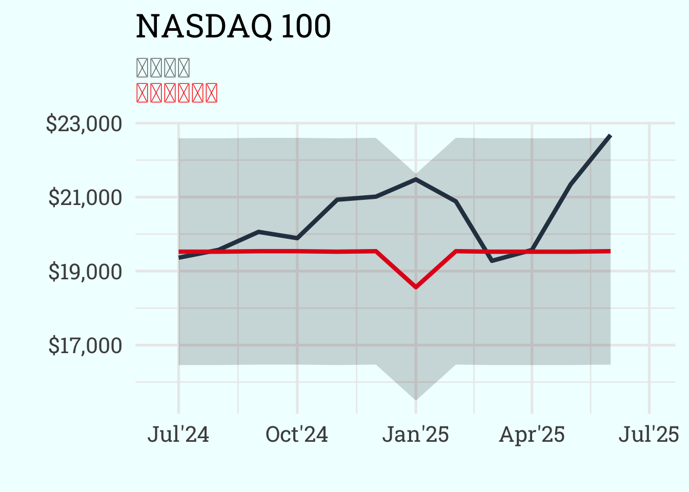
四、竞争算法
XGBoost 的主要竞争对手包括:
1. LightGBM
开发者:微软(2017 年发布)。
特点:
- 基于直方图的决策树构建,速度比 XGBoost 更快。
- 支持 Leaf-wise(按叶子生长)的树生长策略,而不是 XGBoost 的 Level-wise(按层生长)。
- 内存占用更小,适合大规模数据集。
- 适用场景:超大规模数据集、需要快速迭代的场景。
2. CatBoost
开发者:Yandex(2017 年发布)。
特点:
- 自动处理类别特征(无需手动编码)。
- 采用对称树结构,减少过拟合风险。
- 支持 GPU 加速和分布式训练。
适用场景:包含大量类别特征的数据集(如推荐系统、广告点击预测)。
3. Random Forest
特点:
- 基于 Bagging 思想的集成学习算法,并行训练多棵决策树。
- 对异常值和过拟合更鲁棒。
- 计算复杂度较低,但预测精度可能低于 Boosting 算法。
适用场景:快速 baseline 模型、对解释性要求较高的场景。
4. Neural Networks(神经网络)
特点:
- 适用于非结构化数据(如图像、文本、语音)。
- 需要大量数据才能表现良好。
- 计算资源消耗大,训练时间长。
适用场景:深度学习擅长的领域(如计算机视觉、自然语言处理)。
五、算法选择建议
- 数据规模较小:可尝试 Random Forest 或 CatBoost(处理类别特征更方便)。
- 数据规模中等:XGBoost 和 LightGBM 均可,XGBoost 更成熟,LightGBM 速度更快。
- 包含大量类别特征:优先使用 CatBoost。
- 追求极致速度:选择 LightGBM。
- 非结构化数据:考虑神经网络(如 CNN、Transformer)。
XGBoost 的优势在于其高效性、灵活性和广泛的应用场景,尤其在 Kaggle 竞赛和工业界的结构化数据分析中表现突出。